Linear Regression with One Feature

Introduction

Linear regression is one of the simplest and most well understood algorithms in machine learning and will serve as a great starting point to develop our first machine learning model. As hinted by the chapter title, we’re going to build a linear regression algorithm that uses a single variable, or feature. Linear regression that uses a single variable is referred to as univariate linear regression.

As a practical introduction to linear regression, we’ll begin by making predictions intuitively – no math or algorithms will be involved, just a bit of guesswork. We’ll then formalize this intuition by introducing key machine learning concepts and algorithms that underpin linear regression.

Over the next three chapters, we’ll develop increasingly sophisticated machine learning models that predict the price of stocks as a means to apply what we learn towards solving a real-world problem. By the end of this chapter, you will be equipped with all of the tools you will need to build your own linear regression model that will be able to predict the price of stocks.

Intuitive Linear Regression

The first prediction we’re going to make will be an entirely intuitive one, with no math or algorithms involved - just a bit of guesswork. The table below shows the closing price of Apple shares between June 1^st 2023 and June 22^nd 2023. Given this data set, let’s attempt to predict what the value of Apple shares should be on June 26^th 2023.

Table 2-1: Apple share price, June 1^st 2023 to June 22^nd 2023

Date	Closing Price (USD)
1 June 2023	177.25
2 June 2023	180.09
5 June 2023	180.95
6 June 2023	179.58
7 June 2023	179.21
8 June 2023	177.82
9 June 2023	180.57
12 June 2023	180.96
13 June 2023	183.79
14 June 2023	183.31
15 June 2023	183.95
16 June 2023	186.01
20 June 2023	184.92
21 June 2023	185.01
22 June 2023	183.96

Step 1: Plot the data

As a first step, let’s plot the Apple share price data on a graph. The figure below presents a graph of the Apple share price between June 1^st and June 22^nd 2023, with the trading date on the x-axis and the closing price (in US dollars) on the y-axis.

Figure 2-1: Apple share price between June 1 and June 22 2023

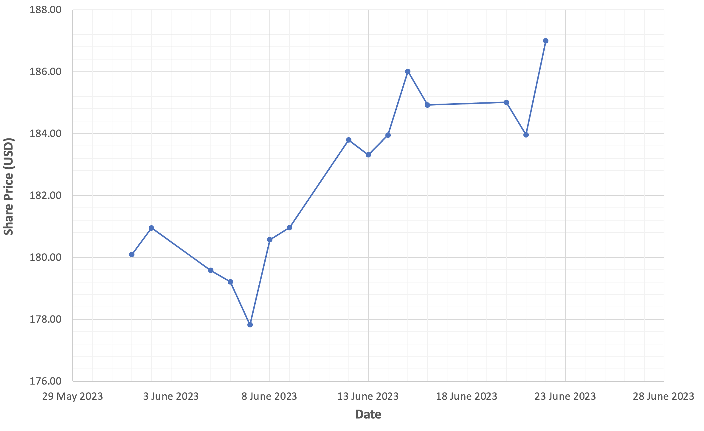
The trading date on the x-axis is the independent variable, and more commonly referred to as a feature in machine learning. The share price on the y-axis is referred to as our dependent variable; this is what machine learning models predict

Step 2: Fit the data

Now that our share price data is plotted on a graph, we simply use our best judgement to draw a straight line that fits the data as best as we can. The figure below shows a red line which appears to provide a reasonable fit for the data.

Figure 2-2: Using judgement to draw a straight line that fits the share price data

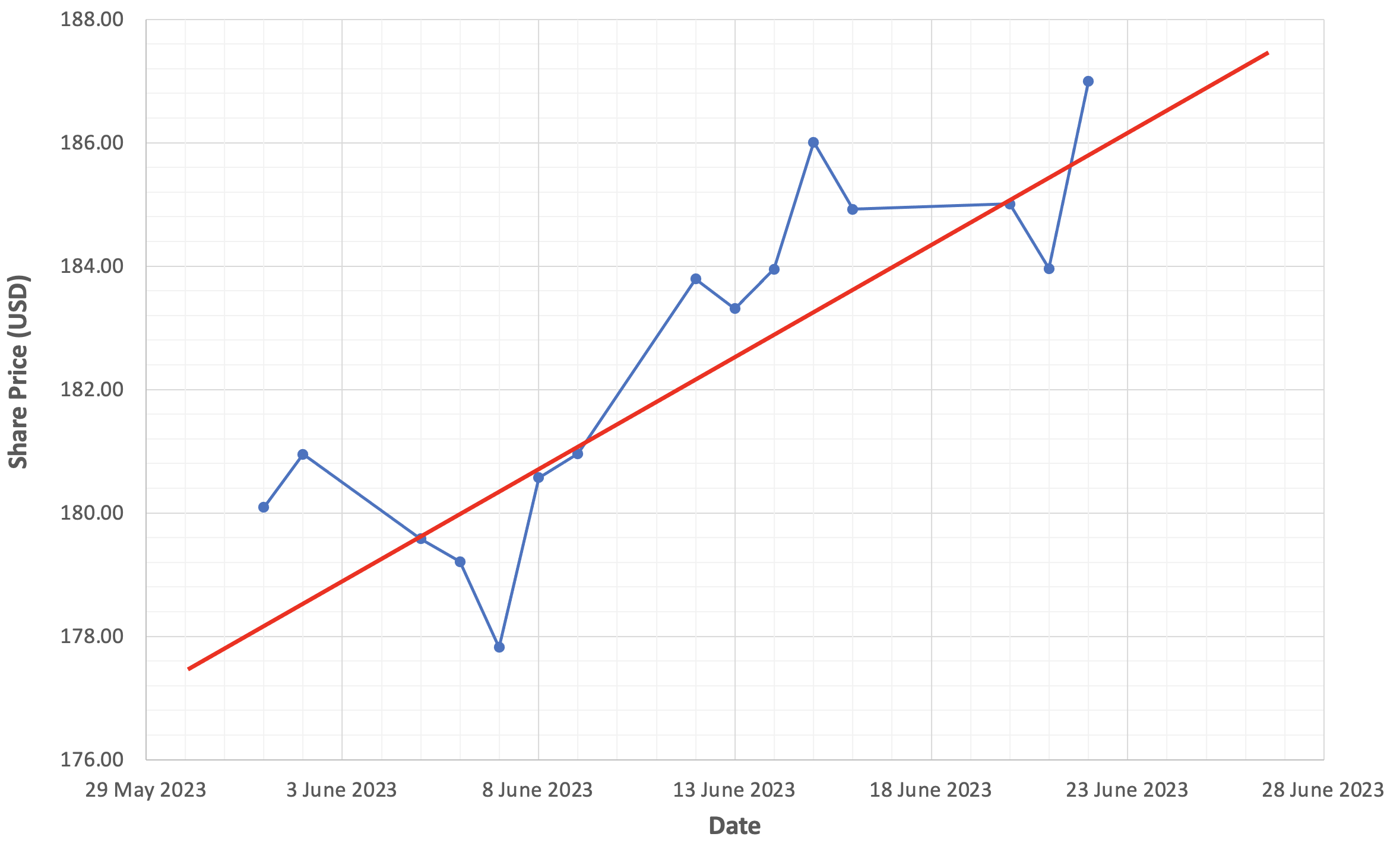
Take a moment to reflect on this image and think about what it means. We’re speculating, or hypothesizing that a relationship exists between the date and Apple’s share price. Further, we’re suggesting that Apple’s share price is influenced by time, but time is not influenced by Apple’s share price.

The red line represents an approximation of the nature of this relationship.

Step 3: Make a prediction

To predict the price of Apple shares on June 26^th 2023, draw a vertical line from the June 26th date located on the x-axis until it intersects with the red line. From the intersection come across to the y-axis to get the predicted price of the Apple shares. The figure below provides you with a visual demonstration of our prediction using green dashed lines.

Figure 2-3: Predicting the price of Apple shares on June 26^th 2023

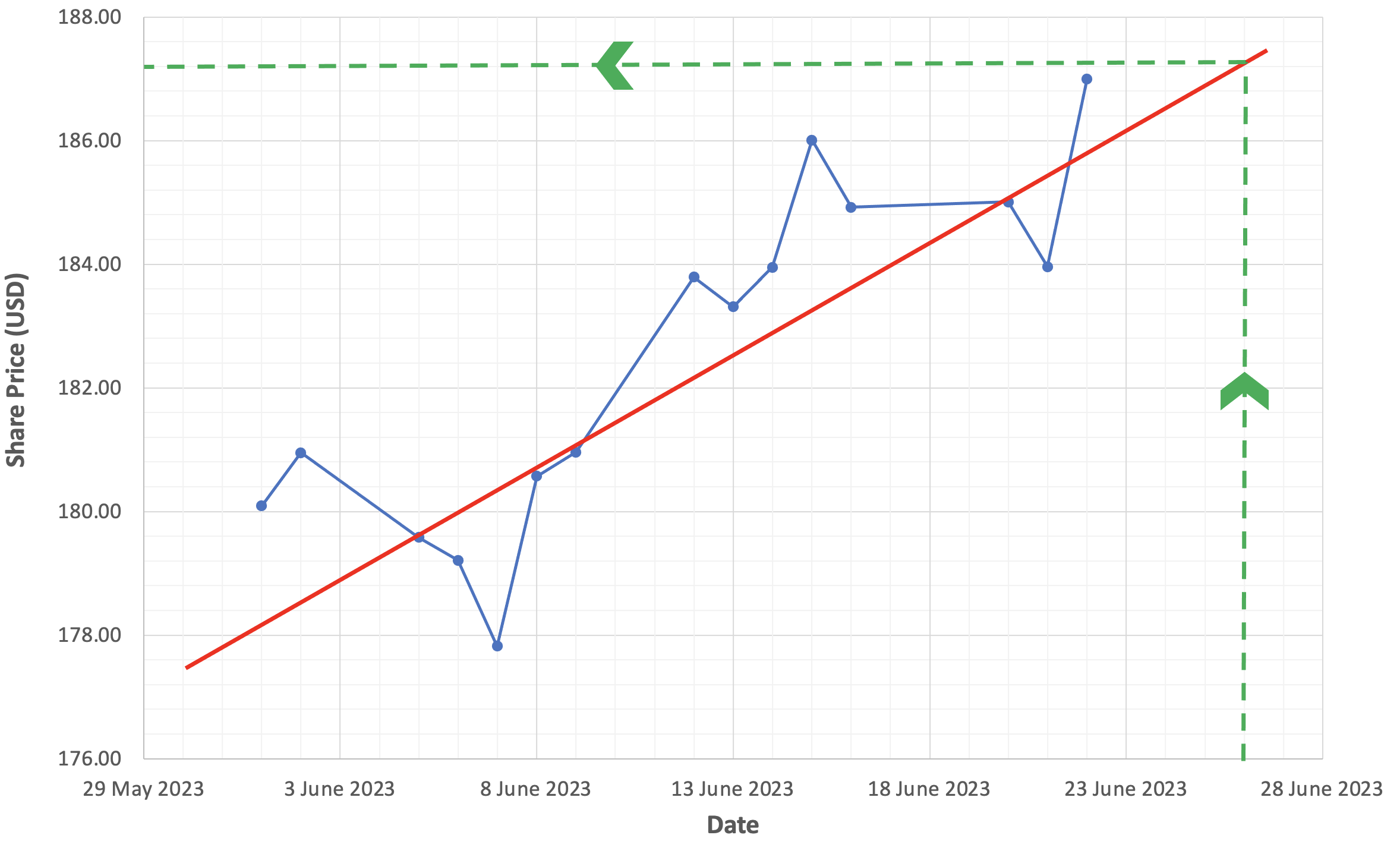
Based on the share price data we collected and analyzed, we can predict that on June 26^th 2023, Apple shares should be valued at approximately $187.40 USD.

Let’s quickly summarize the four steps we just took to make this prediction:

1. We collected data
2. We plotted the data
3. We drew a straight line that best fit the data
4. We used the line to make a prediction

In step 3, we used our judgement to draw a straight line to fit the data as best as we could. For the remainder of this chapter, we’ll go on a journey to replace this judgement with a machine learning algorithm to produce objective, repeatable and mathematically optimized predictions.

The Hypothesis Function

The first step in our journey involves formalizing the concept of the straight red line with a mathematical definition of what the line represents.

The straight red line we drew in Figure 2-2 to fit our share price data is an example of a linear function. Linear functions are optimal for modelling linear relationships. If it’s been a while since you’ve worked with linear functions refer to Chapter 12, Linear Algebra for Machine Learning for a brief introduction to linear functions.

A hypothesis function is a mathematical function that is used to model data and make predictions; this is our machine learning model. In this chapter, we’re using a linear function as our hypothesis function to model and predict share prices. In future chapters, we’ll introduce more advanced functions to model and predict share prices, but our goal for this chapter is to keep things as simple as possible.

The hypothesis function for linear regression is defined as:

$$ h_\theta(x) = \theta_0 + \theta_1x $$

The symbol Θ is called theta, and you’ll see references to theta throughout machine learning literature.

The values Θ₀ and Θ₁ represent the function parameters and are commonly referred to as the model parameters. The purpose of a learning algorithm is to discover optimal values for these parameters. Training a model is the act or process of using a learning algorithm to identify the optimal values for your model’s parameters.

The value x represents our independent variable and is commonly referred to as a model feature.

The Goal of Linear Regression

Now that we’ve defined the hypothesis function we’re going to use to predict Apple share prices, we have enough context to define the goal of linear regression:

Given a training set, produce a hypothesis function h so that h(x) is a good predictor for y.

Put simply, linear regression aims to produce a hypothesis function h whose predictions match observations as closely as possible. To do this, linear regression identifies optimal values for both Θ₀ and Θ₁ to minimize the difference between predictions h(x) and observations y.

More concretely, we can define a good predictor as a hypothesis function that most effectively minimizes the difference between predicted values h(x) and observed values y, for all values of x in a training set t.

The smaller the difference, the better the predictor; the larger the difference, the poorer the predictor. In machine learning, we refer to this difference as the cost, and we train machine learning models to minimize this cost.

The Cost Function

The cost function objectively measures how well a hypothesis function acts as a good predictor for a given training set. It does this by computing the average difference between predicted values h(x) and observed values y, for all values of x in a training set.

Instead of simply presenting the cost function, let’s take the time to derive this function so that you can get an appreciation for how it works as a tool to quantify good predictors.

Deriving The Cost Function

Step 1: Calculate the difference between the predicted value h(x) and the observed value y, for each training instance i in the training set.

$$h(x^{(i)}) - y^{(i)}$$

Step 2: Sum up all of the differences for each instance in the training set. The variable m refers to the size of the training set.

$$\displaystyle \sum _{i=0}^m \left (h (x^{(i)}) - y^{(i)} \right)$$

Step 3: Divide the total difference by the size of the training set to calculate the average difference for the training set.

$$\dfrac {1}{m} \displaystyle \sum _{i=0}^m \left (h (x^{(i)}) - y^{(i)} \right)$$

What we’ve just derived in step 3 is a perfectly usable cost function, but we’re going to make two modifications to simplify a software-based implementation of this function.

First, we are going to square the error component - the difference between the predicted value h(x) and observed value y. Squaring ensures that we always produce a positive number; for example 4² and -4² are both equal to 16. Since the cost function only cares about the magnitude of error, this technique removes a bit of complexity in dealing with positive and negative numbers. We end up with the following cost function:

$$\dfrac {1}{m} \displaystyle \sum _{i=0}^m \left (h (x^{(i)}) - y^{(i)} \right)^2$$

Second, the entire cost function is multiplied by ½ so that the function remains consistent when derivatives of this function are taken. Since the derivative of x² is 2x, multiplying by ½ negates the effect of the exponent.

This is the formal definition of the cost function, which is also referred to as the squared error function or mean error function:

$$\dfrac {1}{2m} \displaystyle \sum _{i=0}^m \left (h (x^{(i)}) - y^{(i)} \right)^2$$

The cost function is conventionally defined as J.

To measure the performance of a hypothesis function, we substitute the reference to the hypothesis function h(x) with the definition of the hypothesis function - in our case, the linear function h(x) = Θ₀ + Θ₁x_i.

After we plug in the hypothesis function, we end up with a cost function that we can use to measure the performance of our linear regression hypothesis function:

$$J(\theta_0, \theta_1) = \dfrac {1}{2m} \displaystyle \sum _{i=0}^m \left (\theta_0 + \theta_1x^{(i)} - y^{(i)} \right)^2$$

We can now express the goal of linear regression in slightly more specific terms - the goal of linear regression is to identify values for the parameters Θ₀ and Θ₁ so that the cost function J(Θ₀, Θ₁) produces the smallest possible value. Put simply, the goal of linear regression is to minimize J(Θ₀, Θ₁).

The Cost Function in Practice

To get a better appreciation of how the cost function works, let’s work through an exercise to calculate and compare the cost of a hypothesis function using different sets of parameters to find out which one would act as the better predictor.

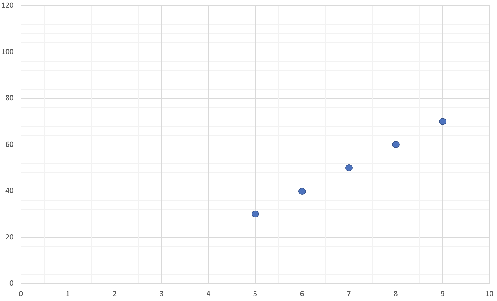
We’ll start the exercise with a simple training set. Table 2-2 below shows the data in our training set and Figure 2-4 below plots our training set on a graph.

Table 2-2: The training set

x	y
5	30
6	40
7	50
8	60
9	70

Figure 2-4: Graph of the training set from Table A

Given the training set we defined above, which hypothesis function would act as a better predictor?

1. A hypothesis function with parameter values 3 and 11
2. A hypothesis function with parameter values 1 and 5

Even though we’re using a simple data set, it might be difficult to answer this question with any degree of confidence. Maybe we’ll get some better insights if we plot these competing functions, so let’s do that now.

Figure 2-5: Comparing two linear regression hypothesis functions

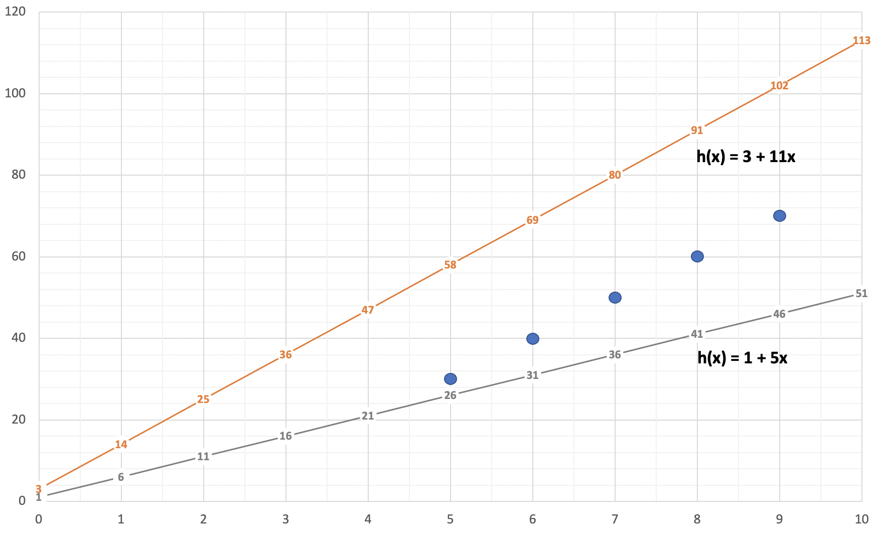
Based purely on observation, Figure 2-5 suggests that the function h(x) = 1 + 5x is likely a better predictor. While I’m now more confident that (2) is the correct answer, let’s calculate the cost of both hypothesis functions and remove all doubt. The tables below show the work to calculate the cost of our competing hypothesis functions.

Table 2-3: Calculating the cost function for h(x) = 1 + 5x

x	Predicted Value	Observed Value	Difference	Squared Difference
5	h(5) = 1 + 5*5 = 26	30	-4	16
6	h(6) = 1 + 5*6 = 31	40	-9	81
7	h(7) = 1 + 5*7 = 36	50	-14	196
8	h(8) = 1 + 5*8 = 41	60	-19	361
9	H(9) = 1 + 5*9 = 46	70	-24	576
Sum of squared differences				1230
Cost function J(1, 5)				123

Table 2-4: Calculating the cost function for h(x) = 3 + 11x

x	Predicted Value	Observed Value	Difference	Squared Difference
5	h(5) = 3 + 11*5 = 58	30	-28	784
6	h(6) = 3 + 11*6 = 69	40	-29	841
7	h(7) = 3 + 11*7 = 80	50	-30	900
8	h(8) = 3 + 11*8 = 91	60	-31	961
9	h(9) = 3 + 11*9 = 102	70	-32	1024
Sum of squared differences				4510
Cost function J(3, 11)				451

By going through this exercise, we’ve been able to objectively demonstrate that (2) is indeed the correct answer. The hypothesis function h(x) = 1 + 5x with a cost of 123 is an objectively and measurably better predictor for this training set than the hypothesis function h(x) = 3 + 11x with a cost of 451.

As an exercise for the reader, come up with values for Θ₀ and Θ₁ that would produce an even better predictor for this training set, and prove it by calculating the cost.

Instead of calculating the cost of hypothesis functions over and over again simply to find the one hypothesis function whose parameters have the lowest cost, wouldn't it be great if there was an algorithm that could automatically find these parameters for us? In the final stage of our data-driven prediction journey, we’ll learn about an algorithm that has the capability to do exactly this.

The Gradient Descent Algorithm

The gradient descent algorithm has broad applicability in machine learning as it offers an efficient means to minimize functions. Before we define the gradient descent algorithm, let’s gain an intuitive understanding of how the algorithm works and an appreciation of its limitations.

The Gradient Descent Hiking Analogy

The gradient descent algorithm is very efficient at discovering local minima - the smallest value of a function in and around a local area of a function. We’ll show that the discovery of local minima, as it turns out, also happens to be an efficient way to discover the optimal values for parameters Θ₀ and Θ₁.

But first, we'll help you get a sense of what local minima are, and how the gradient descent algorithm works to discover them.

Figure 2-6: An introduction to local minima and intuitive gradient descent

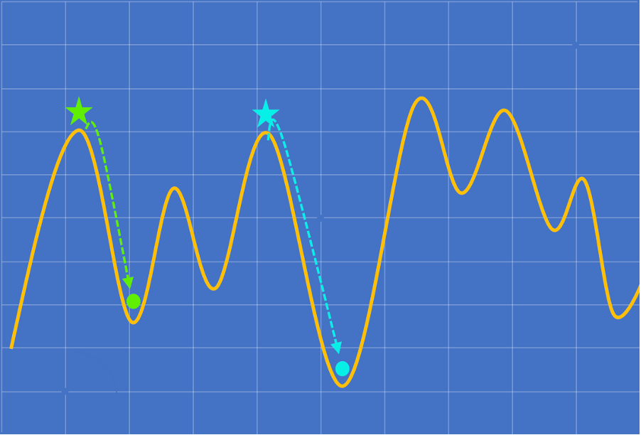
Let’s assume that the function in the above figure represents a side-on view of a mountain range, with your current location on the mountain marked by the green star.

You notice a storm rolling in, and visibility is getting poor. To ride out the storm in safety, you quickly begin making your way down to the base of the mountain. Let’s describe an approach to descend the mountain as a series of simple, logical steps:

1. Look around and find a location that is lower than your current location.
2. Take a step in that direction.
3. Once you reach your new location, repeat steps 1 and 2 until you can no longer find a lower location.

Following approach will bring you, as far as you’re aware, to the base of the mountain represented by the green circle in Figure 2-6.

These three steps provide an intuitive representation of how the gradient descent algorithm works in practice. When we say that gradient descent is efficient at minimizing functions, we’re saying that it’s effective at finding local minima in a function. It does this by algorithmically “descending” the function to find a local minima.

The Limitations of Gradient Descent

There is one limitation of gradient descent that we wanted to point out - had we started this exercise from the blue star, we would have descended to an even lower point on the mountain.

Algorithmically, this implies that gradient descent is sensitive to initial conditions. In other words gradient descent can, and most likely will, produce different results when it is applied against functions with multiple local minima. Consequently, we want to limit the use of gradient descent to functions that have a single, global minima.

Visualizing the Topology of the Cost Function

The linear regression cost function has a single global minima, so it’s well suited to be minimized by the gradient descent algorithm. The reason why these functions produce a single global minima is beyond the scope of this book, but we’ll present a visualization of the function so you can appreciate the “terrain” that the gradient descent algorithm will traverse, and provide you with some insight into what the visualization represents with a thought experiment.

In our introduction to the cost function, we went through a practical exercise to compute the cost of our hypothesis function with two different sets of values for Θ₀ and Θ₁. The results that we computed were as follows:

For Θ₀ = 1 and Θ₁ = 5, we computed J(1, 5) = 123
For Θ₀ = 3 and Θ₁ = 11, we computed J(3, 11) = 451

Let’s imagine plotting these two results on a graph. Since we have three variables (Θ₀, Θ₁ and the cost), we need to plot this data on a graph with x, y and z coordinates. We assign Θ₀ on the x-axis, Θ₁ on the y-axis, and the cost J(Θ₀, Θ₁) on the z-axis. We end up with a three dimensional graph that represents of cost as a function of Θ₀ and Θ₁. At this stage, the graph would consist 2 distinct points sitting in a 3D space.

Let’s assume that we have a lot of free time on our hands, and compute the cost function with slightly different values for Θ₀ and Θ₁ thousands of times, and plot these points on the graph. As you plot this data, a distinct shape will begin to emerge; computing and plotting an arbitrarily large number of these data points would end up producing the concave structure in the figure below.

Figure 2-7: Visualizing cost as a function of Θ₀ and Θ₁

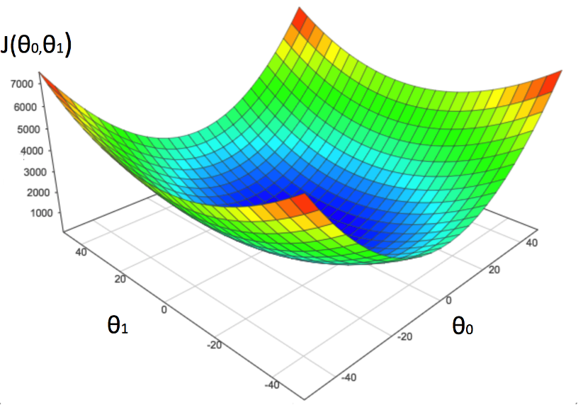
This figure visualizes cost as a function of Θ₀ and Θ₁, and accurately represents the topology or "terrain" that gradient descent will navigate. All linear regression cost functions will end up producing this concave shape, which is why we can use the gradient descent algorithm to minimize linear regression cost functions.

Areas in red represent high costs and are consequently bad predictors. Areas in blue represent low costs and are consequently good predictors. Since the job of gradient descent is to efficiently discover the local minima of a function, it will ultimately discover the most optimal values for Θ₀ and Θ₁, providing us with the best predictor

The Gradient Descent Algorithm

So far we’ve described the gradient descent algorithm intuitively, as three simple steps to traverse down a mountain. We’ll now formalize this intuition by introducing the gradient descent algorithm:

repeat until convergence, for j = 0 and j = 1: {

}

While this definition may initially seem unintuitive, we’ll work to demystify the gradient descent algorithm to show that it’s simply a formal representation of our earlier intuition.

Figure 2-8: The gradient descent algorithm with an overlay of the mountain analogy

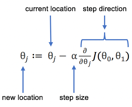
Let’s review some of the new terms introduced in the gradient descent algorithm:

$$ := $$	The expression := means assignment. The assignment ensures that we don’t lose reference to our current location as the algorithm iteratively converges towards the right solution.
$$ \alpha $$	This is the term alpha, also known as the learning rate and defines the size of the step you want to take. We will discuss the learning rate in detail shortly.
$$ \frac{\partial}{\partial \theta_j} J(\theta_0, \theta_1) $$	This term represents the derivative of the cost function and defines the direction of the steps you’re taking. There’s a bit more to unpack here, and we’ll provide more insight about how this term works shortly.

The algorithm instructs us to "repeat until convergence, for j = 0 and j = 1". What does this statement mean?

Whenever you take a step, you’re moving some distance along the x axis (Θ₀) and some distance along the y axis (Θ₀). The gradient descent algorithm needs a practical means to capture and track these two distinct coordinates, so that the algorithm has a reference to where it currently is, and where it needs to move.

The statement for j = 0 and j = 1 is simply shorthand notation used by the gradient descent algorithm to express the fact that we need to capture and store these two distinct variables. Let’s remove the shorthand notation for the time being, and define the gradient descent algorithm in a way that explicitly tracks the Θ₀ and Θ₁ coordinates:

repeat until convergence: {

}

Now let's substitute the reference to the cost function J(Θ₀, Θ₁) with the actual cost function that we defined in the previous section. The gradient descent algorithm can be expressed as:

repeat until convergence: {

}

The last step in the development of our algorithm requires us to take partial derivatives of these functions, which requires some knowledge of multivariate calculus. While you are more than welcome to work through the derivations yourself, we’ve worked through the derivations for you. We end up with the following definition for the gradient descent algorithm:

repeat until convergence: {

}

It took a bit of effort to get here, but we’ve successfully developed our first machine learning algorithm!

We can use this learning algorithm to train our model using the Apple share price data that we introduced at the beginning of this chapter. Gradient descent will discover the most optimal values for Θ₀ and Θ₁, which we inject into our hypothesis function so that it can act as a good predictor for our data.

To close out this chapter, we will discuss convergence in gradient descent and provide some practical guidance on how to effectively manage the gradient descent learning rate.

Convergence in Gradient Descent

When we introduced the gradient descent algorithm we briefly touched on the following term, the derivative of the cost function:

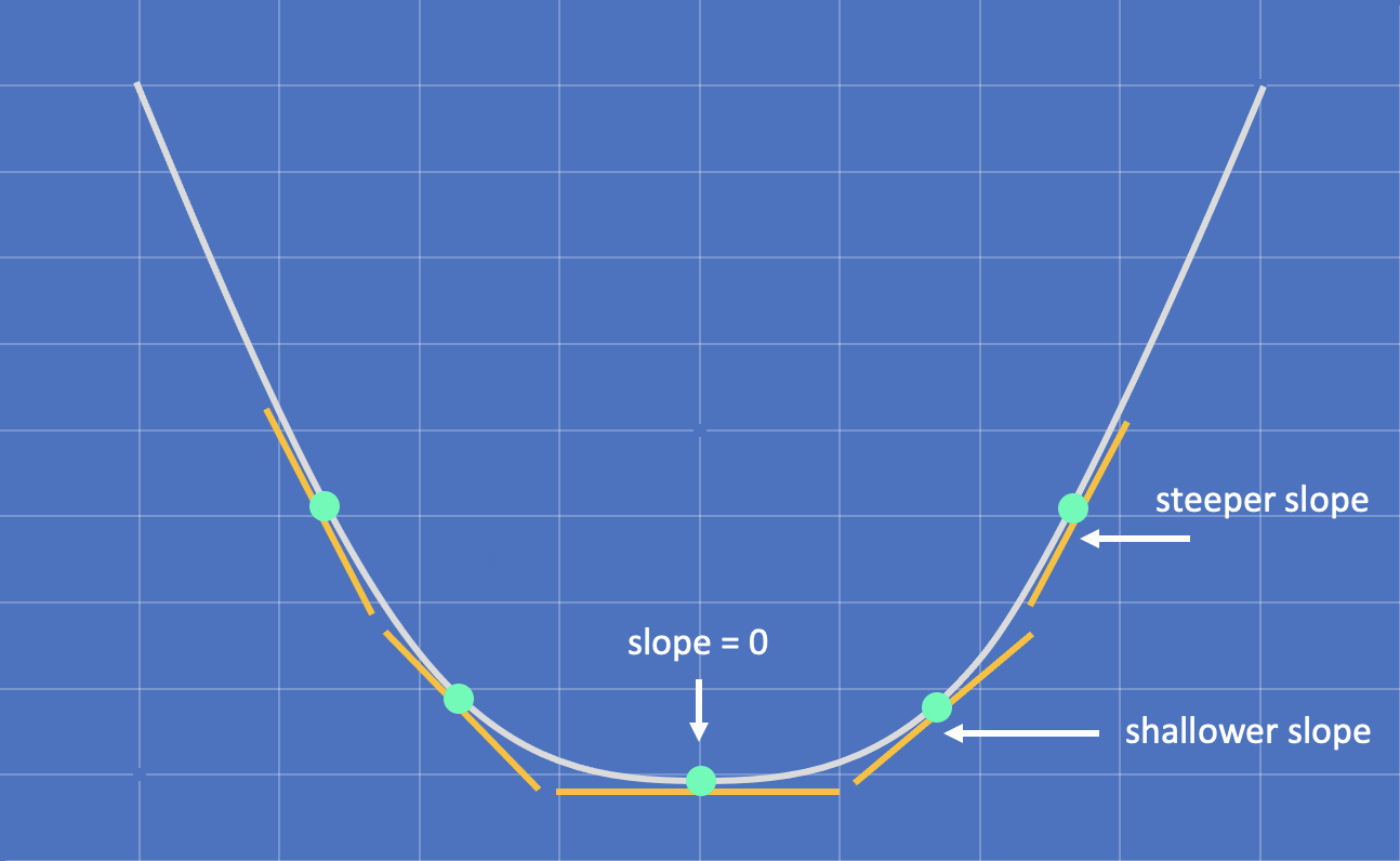
$$ \frac{\partial}{\partial \theta_j} J(\theta_0, \theta_1) $$

The derivative of a cost function computes the slope of the cost function at points Θ₀, Θ₁. Put simply, the slope gives us information about how steep we are at any particular point in a function.

If you refer back to Figure 2-7 where we presented a 3D visual of the cost function, you can see that the edges of the function are steeper than the local minima in the center. Consequently, computing the slope of the cost function at a specific point provides us with an indication of how close we are to finding an optimal solution. The shallower the slope, the closer we are to discovering the local minima.

The figure below presents a cross-section of the 3D cost function that we presented in Figure 8, and shows how the slope of the function successively approaches zero as we approach the local minima.

Figure 2-9: The derivative of the cost function approaches 0 as we approach the local minima.

As we approach the minima, the derivative of the cost function approaches zero; once we reach the global minima, the derivative of the cost function equals zero, and a very useful characteristic of the gradient descent algorithm emerges.

Take our original definition of the gradient descent algorithm (for just one leg; a step in the x direction):

$$ \theta_0 := \theta_0 - \alpha \frac{\partial}{\partial \theta_j} J(\theta_0, \theta_1) $$

Once we reach the minima, the derivative of the cost function is equal to zero, and we end up with:

$$ \theta_0 := \theta_0 - \alpha0 $$

Multiplying the learning rate alpha by zero cancels out this term entirely, and we are left with:

$$ \theta_0 := \theta_0 $$

The key insight here is that when the gradient descent algorithm reaches the minima, the value of Θ₀ becomes immutable; the value will not change with further iterations. Convergence is defined as the incremental progression towards this condition.

In practice, you may not necessarily want to wait for the gradient descent algorithm to reach this condition. You’ll need to pragmatically balance between predictive accuracy and training time to satisfy your specific requirements and use cases.

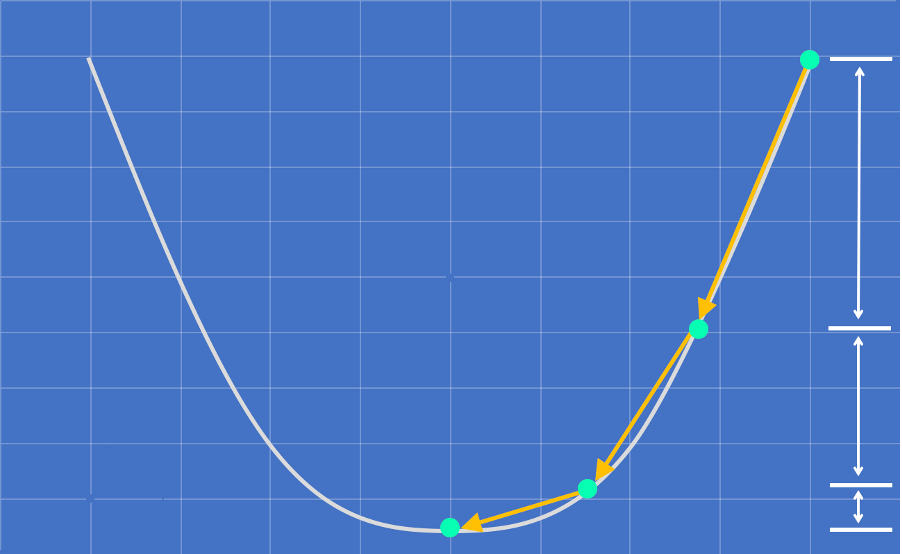
As the gradient descent algorithm approaches the minima, the derivative term will incrementally approach zero after every iteration. Consequently, the algorithm will naturally take incrementally smaller steps as it approaches the minima, and incrementally longer to reach the minima.

The figure below provides a visual of this incremental reduction in step size as the algorithm converges towards the global minima:

Figure 2-10: Incremental reduction in step size as gradient descent converges on the minima

Alpha - The Learning Rate

While the gradient descent algorithm implicitly reduces the step size as it converges on the global minima, the learning rate alpha allows us to explicitly influence the step size. From an implementation perspective, the learning rate alpha is the only adjustable parameter in the gradient descent algorithm, and choosing an appropriate value for alpha ensures that the algorithm finds an optimal solution efficiently. If alpha is set too high, the algorithm may not converge on the most optimal solution; if alpha is set too low, the algorithm may a long time to find the most optimal solution.

Parameters that influence the behaviour of an algorithm such as alpha are referred to as hyperparameters in machine learning.

Figures 2-11 and 2-12 below provide some insight into the behavior of the gradient descent algorithm when the value of alpha is set too high or too low.

Figure 2-11: Linear regression behavior with an aggressive learning rate

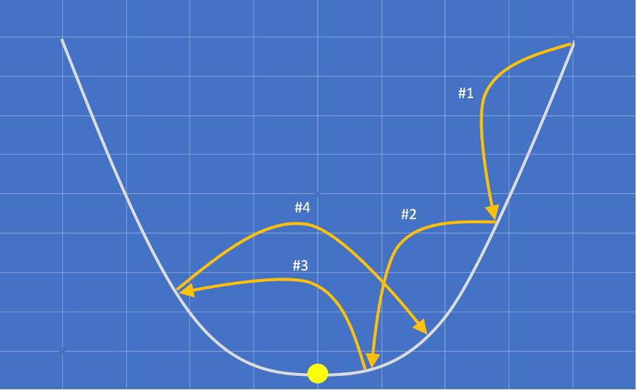
The larger the value of alpha, the larger the steps the gradient descent algorithm will take between each iteration. In iteration #1 and iteration #2, the algorithm takes big steps and gets closer to the minima (the yellow circle). In iteration #3 the algorithm overshoots the minima and iteration #4 begins to diverge from the right solution.

When alpha is set at a high value we risk the possibility of never converging on the minima.

Figure 2-12: Linear regression behavior with a conservative learning rate

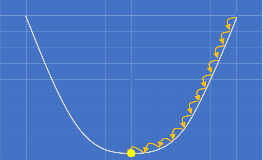
The smaller the value of alpha, the smaller the steps the gradient descent algorithm will take between each iteration. If the learning rate is set conservatively, the gradient descent algorithm will take a larger number of smaller steps, which increases the time it will take to find an optimal solution.

Key Takeaways

The concepts, terminology and algorithms that we’ve introduced in this chapter will lay the groundwork for the development of more sophisticated machine learning algorithms in upcoming chapters. Before you move on to the next chapter, these are the key takeaways that you should be comfortable with.

The Hypothesis Function

The hypothesis function is a machine learning model. Before training, the model will have unoptimized parameter values – in our case, unoptimized values for Θ₀ and Θ₁. The purpose of training a model is to discover the optimal parameter values so that the model acts as a good predictor for the data it’s been trained on. In this chapter, we used a simple linear function as the hypothesis function to model Apple’s share price over the month of June 2023.

The Cost Function

The cost function objectively quantifies how well a model performs against a training data set with respect to specific values, commonly referred to as the parameter weights.

The Gradient Descent Algorithm

Gradient descent is the algorithm we use to train our model. It uses the quantitative performance measurements computed by the cost function to seek and discover the parameter values that produce the lowest cost, which identifies the best predictor for a given data set.

Machine learning algorithms typically have one or many hyperparameters, which are adjustable parameters that are not part of the model itself. The Gradient Descent algorithm has one hyperparameter, the learning rate alpha.

Feature Engineering

Feature engineering is a process that involves selecting, transforming, or creating relevant features from the raw data to improve the performance of a machine learning model. The goal of feature engineering is to enhance a model's ability to capture patterns, relationships, and information within the data, ultimately leading to better predictive outcomes.

We need to apply a technique from feature engineering to transform the date feature from a text representation (i.e. “June 10 2023”) into a numerical representation so that we can train our linear regression model.

There are a number of techniques to transform dates, the most appropriate of which will depend on the characteristics of your data and the problem you’re trying to solve. That said, we’ll broadly describe some of the more common techniques you can employ to transform dates into computational representations.

Feature Extraction

This technique extracts and creates more meaningful features from underlying data. While we’ll provide more concrete examples of feature extraction in the next chapter, the following demonstrates how the string “June 10 2023” can expressed as three distinct features:

“June 10 2023” = [6, 10, 2023]

Timestamp Encoding

This technique converts a date into a timestamp. The following example demonstrates how the string “June 10 2023” is expressed as a timestamp:

“June 10 2023” = 1686355200000

Ordinal Encoding

This technique converts a date into ordinal values by assigning a unique number to each element of the date. The following example demonstrates how the string “June 10 2023” is expressed as an ordinal value:

“June 10 2023” = 6102023

Periodic Encoding

This technique converts a date into sine and cosine components to preserve the cyclical nature of a date and is commonly used to capture cyclic patterns, such as seasonality. The following example demonstrates how the string “June 10 2023” is expressed as sine and cosine components:

“June 10 2023” = ~0.985 (sine component), ~0.174 (cosine component)

Elapsed Time

This technique calculates the number of days (or suitable time units) that have elapsed since a reference date. If we use Apple’s IPO date of December 12 1980 as an example, this is how June 10 2023 would be expressed as the number of days since the IPO date:

“June 10 2023” = 15520

Feature Engineering in Practice

Due to its broad applicability in machine learning, you’ll likely find that feature extraction is the most useful and commonly used transformation technique from the list we’ve described. That said, the univariate linear regression model only supports one feature, so we won’t be able to use feature extraction to transform the date feature into a more meaningful collection of features.

In our implementation of the univariate linear regression on GitHub, we’ve elected to use the timestamp encoding technique simply because the technique is straightforward to implement, and more capable machine learning models that we build in future chapters won’t have the same constraints as we have now.

Build the Univariate Linear Regression Model

We’ve published an implementation of the univariate linear regression model on GitHub.

If you would like to implement, train and run this linear regression model yourself, feel free to use the source code as a reference and run the software to see how training and running the model works in practice. Documentation related to building, training and running the model can be found on GitHub as well.

https://github.com/build-thinking-machines/univariate-linear-regression