Linear Algebra for Machine Learning
Introduction
Linear algebra is a foundational branch of mathematics that provides a powerful framework for understanding and solving a wide range of problems in various fields, from physics and engineering to computer science and economics. It provides us with tools to model, analyze, and solve complex problems by simplifying them into structured mathematical constructs, making it a fundamental area of study for anyone delving into the sciences or engineering.
At its core, linear algebra deals with the study of vectors, vector spaces, and linear transformations. Vectors are quantities that possess both magnitude and direction and can be represented as ordered lists of numbers. A vector space is a set of vectors that obeys specific mathematical rules, such as closure under addition and scalar multiplication. Linear transformations are functions that map vectors from one space to another while preserving key vector space properties.
The purpose of this chapter is to provide you with a broad overview of linear algebra, with a focus on specific topics that will be relevant to your understanding of the machine learning algorithms introduced in this book.
Linear Functions
A linear function is a mathematical function whose graph is a straight line, which takes the form:
$$ y = f(x) = a + bx $$The variable y is referred to as the dependent variable, x is referred to as the independent variable, a is referred to as the y-intercept, and b is referred to as the slope or coefficient of x. The y-intercept and slope are known as constants of the function.
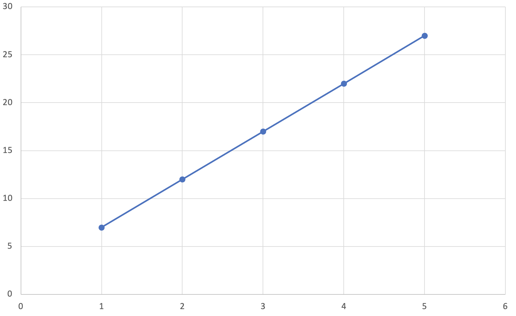
Let’s work through a concrete example by graphing a linear function using a y-intercept of 2 and a slope of 5:
$$ y = f(x) = 2 + 5x $$| x | f(x) = 2 + 5x | y |
| 1 | f(1) = 2 + 5*1 | 7 |
| 2 | f(2) = 2 + 5*2 | 12 |
| 3 | f(3) = 2 + 5*3 | 17 |
| 4 | f(4) = 2 + 5*4 | 22 |
| 5 | f(5) = 2 + 5*5 | 27 |
Now that we’ve calculated y for each value of x, let’s plot each of the (x, y) pairs on a graph and draw a line through each pair. Doing so produces a straight line on a graph, as shown in the figure below.
Matrices, Vectors and Scalars
By the end of this section you should understand what matrices, vectors and scalars are and have the ability to apply simple mathematical operations to them.
Matrices
A matrix is a rectangular array of numbers arranged into rows and columns. Each number in a matrix is referred to as a matrix element or entry. The dimensions of a matrix specify the number of rows and columns in that order.
The following matrix has 3 rows and 4 columns; we refer to this matrix as a 3 x 4 matrix.
$ \begin{bmatrix}2 & 1 & 8 & 2\\5 & 8 & 2 & 6\\9 & 0 & 4 & 3\end{bmatrix} $The following matrix has 2 rows and 5 columns; we refer to this matrix as a 2 x 5 matrix.
$ \begin{bmatrix}7 & 8 & 0 & 9 & 1\\3 & 8 & 6 & 4 & 0\end{bmatrix} $A specific element in a matrix is identified by its row and column number. For example, take the following 2 x 3 matrix G.
$ G = \begin{bmatrix}11 & 13 & 56\\\color{green}23 & 19 & 30\end{bmatrix} $The element g2,1 refers to the element in the second row and first column, highlighted in green above. In this case, we would say that:
g2,1 = 23
More generally, the element in row i and column j in matrix A is denoted ai,j.
Vectors
A vector is a matrix with either one row or one column. A vector with exactly one column is called a vector, while a vector with exactly one row is called a row vector.
The following vector is a 4 x 1 matrix that has one column and four rows.
$ C = \begin{bmatrix}2\\3\\4\\6\end{bmatrix} $The following row vector is a 1 x 4 matrix that has one row and four columns.
$ R = \begin{bmatrix}5 & 6 & 7 & 8\end{bmatrix} $Scalars
A scaler is a matrix with exactly one row and one column; in other words, a scaler is simply a 1 x 1 matrix that contains exactly one element. The following scalar has exactly one element, and more conventionally we’ll omit the square brackets associated with matrices and simply refer to the scalar value itself.
$ A = \begin{bmatrix}5\end{bmatrix} = 5 $Matrix Addition
So long as we have two matrices with identical dimensions, we can add matrices in a similar fashion to how we would add two numbers. Given two matrices A and B:
$ A = \begin{bmatrix}2 & 1\\3 & 5\end{bmatrix} \hspace{0.5cm} B = \begin{bmatrix}3 & 3\\1 & 2\end{bmatrix} $We can find the sum of the matrices A and B by adding their corresponding entries together. The following example shows how to sum matrix A and B:
$ A + B = \begin{bmatrix}\color{green}2 & \color{green}1\\\color{green}3 & \color{green}5\end{bmatrix} + \begin{bmatrix}\color{blue}3 & \color{blue}3\\\color{blue}1 & \color{blue}2\end{bmatrix} = \begin{bmatrix}\color{green}2+\color{blue}3 & \color{green}1+\color{blue}3\\\color{green}3+\color{blue}1 & \color{green}5+\color{blue}2\end{bmatrix} = \begin{bmatrix}5 & 4\\4 & 7\end{bmatrix} $Matrix Subtraction
So long as we have two matrices with identical dimensions, we can subtract matrices in a similar fashion to how we would subtract two numbers. Given two matrices A and B:
$ A = \begin{bmatrix}2 & 1\\3 & 5\end{bmatrix} \hspace{0.5cm} B = \begin{bmatrix}3 & 3\\1 & 2\end{bmatrix} $We can find the difference between matrices A and B by subtracting their corresponding entries together. The following example shows how to subtract matrix B from matrix A:
$ A - B = \begin{bmatrix}\color{green}2 & \color{green}1\\\color{green}3 & \color{green}5\end{bmatrix} - \begin{bmatrix}\color{blue}3 & \color{blue}3\\\color{blue}1 & \color{blue}2\end{bmatrix} = \begin{bmatrix}\color{green}2-\color{blue}3 & \color{green}1-\color{blue}3\\\color{green}3-\color{blue}1 & \color{green}5-\color{blue}2\end{bmatrix} = \begin{bmatrix}-1 & -2\\2 & 3\end{bmatrix} $Scalar Multiplication
The term scalar multiplication refers to the product of a scalar and a matrix. Each element in a matrix is multiplied by the scalar, so this process works in a similar fashion to how we would multiply two numbers.
$ 2 \cdot \begin{bmatrix}\color{green}1 & \color{green}2\\\color{green}3 & \color{green}4\end{bmatrix} = \begin{bmatrix}2 \cdot\color{green}1 & 2 \cdot \color{green}2\\2 \cdot \color{green}3 & 2 \cdot \color{green}4\end{bmatrix} = \begin{bmatrix}2 & 4\\6 & 8\end{bmatrix} $Vector Multiplication
The term vector multiplication refers to the product of a vector and a matrix. You can only apply vector multiplication when the number of rows in the vector matches the number of columns in a matrix.
To calculate the product of a vector matrix multiplication, you take the product of the first element of the vector and the first element of the first row in the matrix, then take the product of the second element of the vector and the second element of the first row in the matrix, and sum the two products together. Repeat this process for each row in the matrix.
$ \begin{bmatrix}\color{blue}1\\\color{green}2\end{bmatrix} \cdot \begin{bmatrix}1 & 2\\3 & 4\end{bmatrix} = \begin{bmatrix}\color{blue}1 \color{black}\cdot 1 + \color{green}2 \color{black}\cdot 3\\\color{blue}1 \color{black}\cdot 2 + \color{green}2 \color{black}\cdot 4\\\color{blue}1 \color{black}\cdot 6 + \color{green}2 \color{black}\cdot 6\end{bmatrix} = \begin{bmatrix}6\\10\\17\end{bmatrix} $Matrix Multiplication
The term matrix multiplication refers to the product of two matrices. You can only apply matrix multiplication when the number of columns in the first matrix matches the number of rows in the second matrix. As an example, let’s multiply matrices A and B, defined as follows:
$ A = \begin{bmatrix}2 & 3 & 4\\5 & 6 & 7\end{bmatrix} \hspace{0.5cm} B = \begin{bmatrix}1 & 4\\2 & 5\\3 & 6\end{bmatrix} $To perform this multiplication, we’ll convert the matrix B into two distinct column vectors. We’ll perform two vector multiplications, and then combine the results. The formula below visualizes the approach we’re going to take:
$ A \cdot B = \begin{bmatrix}2 & 3 & 4\\5 & 6 & 7\end{bmatrix} \cdot \begin{bmatrix}\color{blue}1 & \color{blue}4\\\color{green}2 & \color{green}5\\\color{red}3 & \color{red}6\end{bmatrix} = \begin{bmatrix}2 & 3 & 4\\5 & 6 & 7\end{bmatrix} \cdot \begin{bmatrix}\color{blue}1\\\color{green}2\\\color{red}3\end{bmatrix} (+) \begin{bmatrix}2 & 3 & 4\\5 & 6 & 7\end{bmatrix} \cdot \begin{bmatrix}\color{blue}4\\\color{green}5\\\color{red}6\end{bmatrix} $We perform vector multiplication on the first vector and produce our first 2 x 1 vector product:
$ \begin{bmatrix}2 & 3 & 4\\5 & 6 & 7\end{bmatrix} \cdot \begin{bmatrix}\color{blue}1\\\color{green}2\\\color{red}3\end{bmatrix} = \begin{bmatrix}(\color{blue}1\color{black}\cdot2) + (\color{green}2\color{black}\cdot3) + (\color{red}3\color{black}\cdot4)\\(\color{blue}1\color{black}\cdot5) + (\color{green}2\color{black}\cdot6) + (\color{red}3\color{black}\cdot7)\end{bmatrix} = \begin{bmatrix}2 + 6 + 12\\5 + 12 + 21\end{bmatrix} = \begin{bmatrix}20\\38\end{bmatrix} $We perform vector multiplication on the second vector and produce our second 2 x 1 vector product:
$ \begin{bmatrix}2 & 3 & 4\\5 & 6 & 7\end{bmatrix} \cdot \begin{bmatrix}\color{blue}4\\\color{green}5\\\color{red}6\end{bmatrix} = \begin{bmatrix}(\color{blue}4\color{black}\cdot2) + (\color{green}5\color{black}\cdot3) + (\color{red}6\color{black}\cdot4)\\(\color{blue}4\color{black}\cdot5) + (\color{green}5\color{black}\cdot6) + (\color{red}6\color{black}\cdot7)\end{bmatrix} = \begin{bmatrix}8+15+24\\20+30+42\end{bmatrix} = \begin{bmatrix}47\\92\end{bmatrix} $We combine the results of the vector products which results in a 2 x 2 matrix with the final result of the matrix multiplication.
$ A \cdot B = \begin{bmatrix}2 & 3 & 4\\5 & 6 & 7\end{bmatrix} \cdot \begin{bmatrix}1 & 4\\2 & 5\\3 & 6\end{bmatrix} = \begin{bmatrix}20 & 47\\38 & 92\end{bmatrix} $Transpose of a Matrix
If matrix A is an R x C matrix, then its transpose, denoted by AT is a C x R matrix where the columns of AT are equal to the rows of A.
To transpose a matrix, take the first row of matrix A and turn it into the first column of matrix AT, then take the second row of matrix A and turn it into the second column of matrix AT, and continue this process until you’ve transposed all of the rows in matrix A.
The following two examples demonstrate how to transpose a matrix.
$ A = \begin{bmatrix}\color{green}2 & \color{green}1\\\color{blue}4 & \color{blue}5\end{bmatrix} \hspace{0.5cm} A^T = \begin{bmatrix}\color{green}2 & \color{blue}4\\\color{green}1 & \color{blue}5\end{bmatrix} $$ A = \begin{bmatrix}\color{green}1 & \color{green}2\\\color{blue}3 & \color{blue}4\\\color{red}5 & \color{red}6\end{bmatrix} \hspace{0.5cm} A^T = \begin{bmatrix}\color{green}1 & \color{blue}3 & \color{red}5\\\color{green}2 & \color{blue}4 & \color{red}6\end{bmatrix} $
Combining Matrix Operations
Let’s apply what we’ve learned so far and work through an example that combines both transposing and multiplying matrices. Given the vectors θ and X below, what is the result of θTX?
$ \theta = \begin{bmatrix}1\\2\\3\\4\end{bmatrix} \hspace{0.5cm} X = \begin{bmatrix}3\\4\\5\\5\end{bmatrix} $First, we take the transpose of the vector θ and we end up with the following row vector:
$ \theta = \begin{bmatrix}1\\2\\3\\4\end{bmatrix} \hspace{0.5cm} \theta^T = \begin{bmatrix}1 & 2 & 3 & 4\end{bmatrix} $Now we can take the product of vectors θT and X:
$ \theta^TX = \begin{bmatrix}1 & 2 & 3 & 4\end{bmatrix} \cdot \begin{bmatrix}3\\4\\5\\5\end{bmatrix} = [(1 \cdot 3) + (2 \cdot 4) + (3 \cdot 5) + (4 \cdot 5)] = 46 $