Polynomial Regression

Introduction

In the previous two chapters, we’ve developed linear regression models to predict the price of Apple shares. Given that financial markets (including the movement of Apple’s share price) are nonlinear in nature, it stands to reason that a nonlinear regression model should act as a significantly better predictor compared to a linear regression model.

In this chapter, we’ll develop our first nonlinear regression model using Polynomial Regression to predict the price of Apple shares. Polynomial regression is a technique that allows you to model nonlinear relationships using polynomial functions.

A key feature of polynomial regression is its use of the linear regression hypothesis function, cost function and gradient descent algorithm. Polynomial regression leverages all of the linear regression machinery that we introduced in the previous chapter.

Instead of developing new functions or algorithms, we’ll make use of feature engineering to encode or express polynomial behaviour in a training set. It’s a simple yet powerful technique to model complex relationships.

Polynomial Functions

Polynomial functions are widely used in mathematics, science, engineering, and various other fields to model and describe relationships and patterns due to their versatility and ability to represent a wide range of functions.

Linear regression models relationships between features and dependent variables using a linear function. In contrast, polynomial regression models relationships between features and dependent variables using a polynomial function. The key characteristic of nonlinear regression is that relationships are modelled as a nonlinear combination of features, where the degree of a polynomial determines the level of nonlinearity in the model.

To get a better sense of what a polynomial function is, let’s take a look at a few examples of different polynomial functions. In Figure 4-1 below we present three different polynomial functions, including a graph of the function and its definition.

Figure 4-1: An overview of polynomial functions

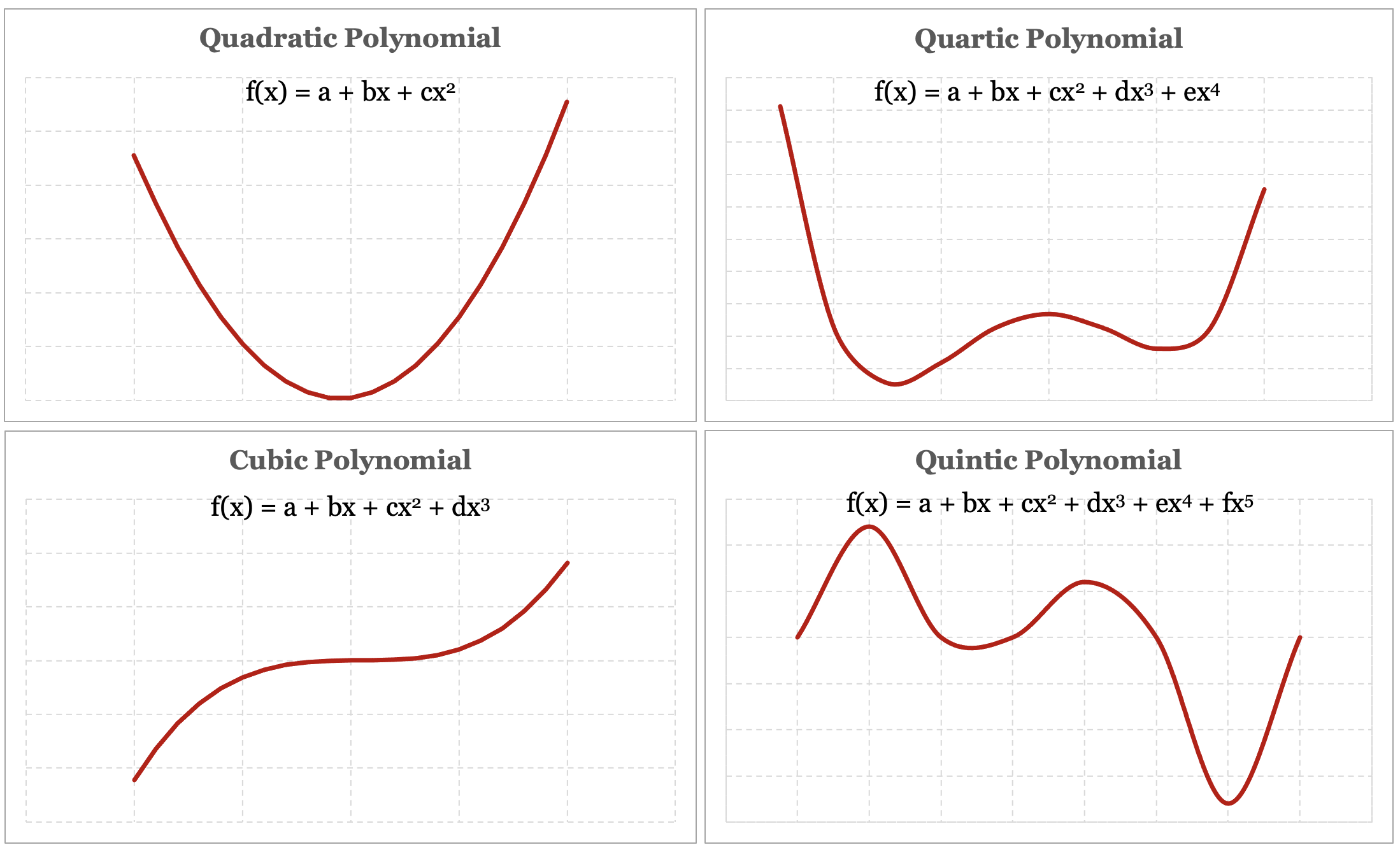
This is an illustrative example of the versatility of polynomial functions, and their ability to represent a wide array of functions. It also reinforces the idea that the degree of the polynomial determines the level of nonlinearity of a model – a fourth-degree quartic polynomial has a greater ability to curve and bend compared to a second-degree quadratic polynomial.

Comparing Linear and Polynomial Models

Now that we have a better understanding of what polynomial functions are and how they behave, let’s get a more intuitive understanding of why polynomial regression may be a better predictor than linear regression for nonlinear systems.

Figure 4-2 below should look familiar; it shows how we originally modelled Apple’s share price using a linear function in Chapter 2.

Figure 4-2: Modelling Apple’s share price using a linear function

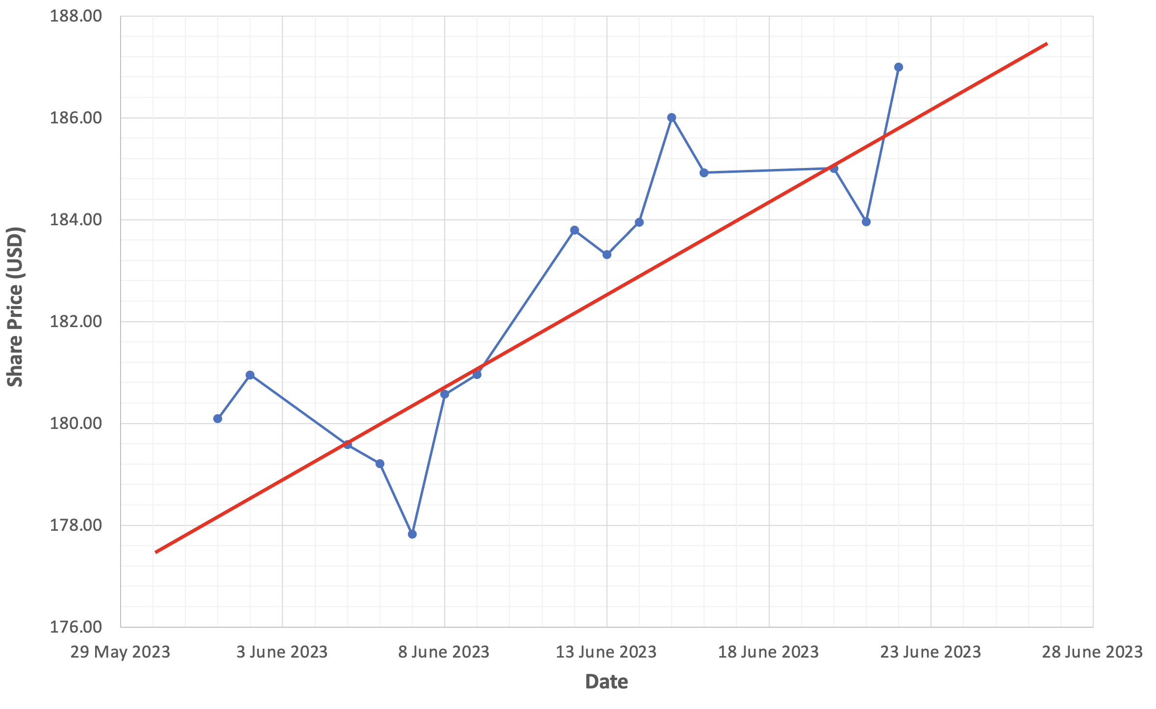
The linear function fails to model or “capture” the dynamic properties inherent in the movement of Apple’s share price. Since linear functions have no ability to bend or curve, linear regression models will struggle to identify and discover underlying relationships in nonlinear systems. As a consequence, linear regression models generally act as poor predictors of nonlinear systems.

Now compare this graph with Figure 4-3 below, where we model Apple’s share price using a fifth-degree polynomial function.

Figure 4-3: Modelling Apple’s share price using a fifth-degree polynomial function

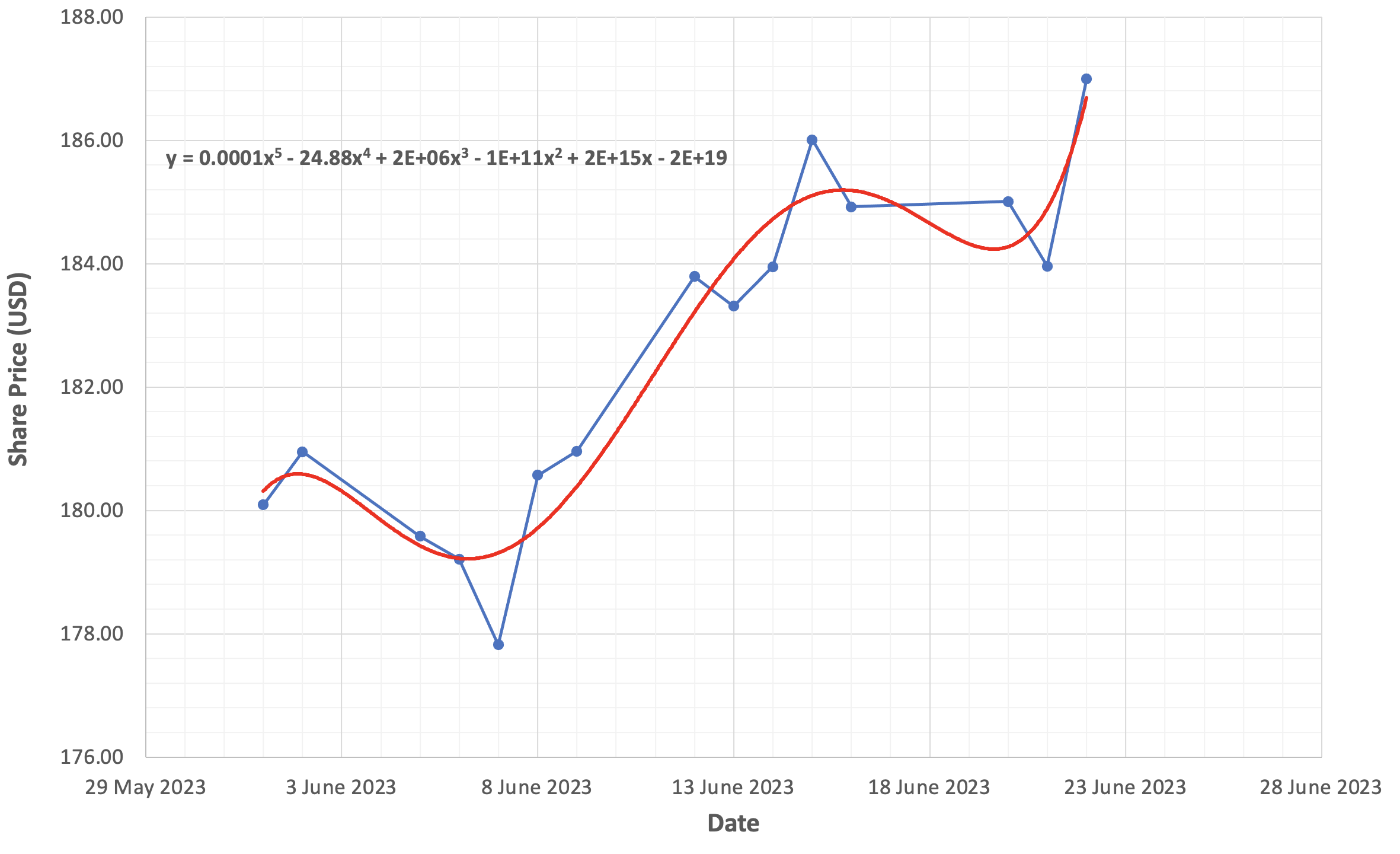
Note how well this polynomial function appears to model the dynamics of Apple’s share price compared to the linear function. Since polynomial functions can bend and curve, they have the ability to “capture” nonlinear system behaviours and characteristics. The figure above also includes the fifth-degree polynomial equation used to graph the function.

This polynomial function seems to fit Apple’s share price quite well...perhaps a bit too well. Due to the inherent extensibility and flexibility of polynomial functions, you need to be aware of both overfitting risk and underfitting risk when you’re modelling domains with polynomial functions.

Overfitting Risk

Overfitting occurs when you use a polynomial function whose degree is too high for your data. This can result in a model that fits the training data extremely well, capturing noise and random fluctuations in the data. Such a model is likely to perform poorly on new, unseen data because it has effectively memorized the training data rather than learning the underlying relationships. Overfit models tend to have overly complex curves that do not generalize well.

Underfitting Risk

Underfitting, on the other hand, occurs when you use a polynomial function whose degree is too low to capture the underlying relationship in the data. An underfit model will have a simple, linear shape and will not adequately account for the nonlinear dynamics in the data. As a result, it will perform poorly on both the training data and new data because it cannot capture the underlying relationship.

Risk Management Techniques

In practice, overfitting risk is the most significant risk when you’re working with higher-order polynomial functions. Later on in this chapter, we’ll introduce regularization as a means to mitigate overfitting risk with higher-order functions.

Feature Engineering with Polynomial Functions

Polynomial regression uses feature engineering to encode or express polynomial behaviour directly in a training set. Once you’ve transformed your data using this technique, you can leverage all of the machinery of multivariate linear regression to train your model.

Let’s work through a simple exercise to get a better understanding of how this feature engineering technique works in practice. To keep things simple, let’s assume that we want to predict Apple’s share price using a single feature, the daily trading volume. Table 4-1 below shows the simple training set that we’re starting with.

Table 4-1: Simple training set

Date	Volume	Close
...	...	...
...	...	...

A conventional linear hypothesis function to capture the volume as a single feature is defined as:

$$ h_\theta(x) = \theta_0x_0 + \theta_1x_1 $$ $$ h_\theta(x) = \theta_0(1) + \theta_1(volume) $$

We believe that a third-degree cubic polynomial function will be a better fit for Apple’s share price. A hypothesis function using a cubic polynomial is defined as:

$$ h_\theta(x) = \theta_0x_0 + \theta_1x_1 + \theta_2x_2^2 + \theta_3x_3^3 $$

While this hypothesis function may be a better model for our data, we can’t plug it into the machinery of linear regression. We remove the exponents from the polynomial function to “collapse” it into a linear function and introduce two new features – volume² and volume³.

$$ h_\theta(x) = \theta_0x_0 + \theta_1x_1 + \theta_2x_2 + \theta_3x_3 $$ $$ h_\theta(x) = \theta_0(1) + \theta_1(volume) + \theta_2(volume^2) + \theta_3(volume^3) $$

There’s no difference between a polynomial function that squares and cubes data, versus a linear function that consumes squared and cubed data.

In practice, we add two new columns to our training set called Volume² and Volume³. We populate the Volume² column with the squared value of the volume and we populate the Volume³ with the cubed value of the volume.

Table 4-2: Simple training set with the volume² and volume³ features added

Date	Volume	Volume2	Volume3	Close
...	...	...	...	...
...	...	...	...	...

In effect, we’ve encoded the behaviour of a polynomial function within our data set. This technique allows us to model nonlinear systems while leveraging the mechanics of linear regression.

It’s important to note that this technique is not limited to creating new exponentiated features. For example, we can define a hypothesis function with the following features:

$$ h_\theta(x) = \theta_0(1) + \theta_1(volume) + \theta_2(\sqrt{volume}) + \theta_3(tanh(volume)) $$

This feature engineering technique provides you with innumerable ways to create new features to model complex domains.

With so many ways to create new features, how might you select optimal features for a model? Principal Component Analysis is a dimensionality reduction technique that is commonly used for feature selection and can help you select features for your model. We’ll introduce Principal Component Analysis in Chapter 8.

Regularization

You can think about bias as the degree to which data can influence a function.

For example, a linear function will never bend nor flex in the presence of data. If you gave them a personality, linear functions are a bit stubborn; they have their own preconceived notion that all relationships are linear, and no amount of data is going to change their opinion. Linear functions have a high bias, as they are not strongly influenced by data. Functions with high bias are prone to underfitting.

A polynomial function, on the other hand, does have the ability to bend and flex in the presence of data. The higher the degree of the polynomial, the greater its ability to bend and flex, and the more susceptible it is to being influenced by data. High-degree polynomials have low bias and are influenced by data to the extent that their goal can quietly and unintentionally transition from learning to simply fitting. Functions with low bias are consequently prone to overfitting. This is a behaviour that we want to avoid and where regularization can help.

Regularization is a technique that moderates or dampens the effects of higher-order polynomial terms in a polynomial function. Many machine learning algorithms will offer regularized versions so you can train models using polynomial and higher-degree data sets. It’s also a technique that involves balance; we want to dampen the effects of higher-order terms to reduce overfitting, but not to the extent that we induce underfitting.

To provide you with some intuition about how regularization works, let’s revisit the fifth-degree polynomial function we used to model Apple’s share price.

$$ h_\theta(x) = \theta_0x_0 + \theta_1x_1 + \theta_2x_2^2 + \theta_3x_3^3 + \theta_4x_4^4 + \theta_5x_5^5 $$

The last two terms of the fifth-degree polynomial have relatively low bias and are consequently at the greatest risk of inducing underfitting behaviour. However, if we choose to make the parameter values θ_4 and θ_5 incredibly small, we could minimize or effectively negate their impact, and consequently reduce underfitting risk. This is how regularization works to reduce underfitting risk. In practice, regularization encourages gradient descent to produce a trained model whose parameter values are minimized.

Ridge Regression

Ridge regression, also known as L2 Regularization is a regularization technique that adds a penalty to the cost function. Below we present a version of the cost function with the regularization term added in blue:

$$ J(\theta) = \dfrac {1}{2m} \displaystyle \sum _{i=0}^m \left (\theta^Tx^{(i)} - y^{(i)} \right)^2 + \color{blue}\lambda\sum _{j=1}^n \theta_j^2 $$

Let’s spend a bit of time to unpack this new term. The summation operator sums the square of the parameter values in our model except for parameter θ₁ - this parameter is commonly excluded since its paired variable x₁ conventionally has a default value of 1. The effect of including or excluding it is negligible. Squaring each parameter ensures that the values of each parameter are positive. As a concrete example, this is what the summation operation would look like with the fifth-order polynomial function we used to model Apple’s share price.

$$ \lambda\sum _{j=1}^n \theta_j^2 = \theta_1x_1 + \theta_2x_2^2 + \theta_3x_3^3 + \theta_4x_4^4 + \theta_5x_5^5 $$

This term penalizes the cost function more as the combined value of the parameters increases and penalizes the cost function less as the combined value of the parameters decreases.

The other element in the regularization term is lambda λ, also known as the regularization parameter. This is another example of a hyperparameter like the learning rate alpha. The purpose of the regularization parameter is to moderate and manage the contention between the cost function, whose goal is to fit the training data as best as possible, and the regularization term, whose goal is to keep parameters small.

If lambda is set too high, we might end up with parameters that are close to zero, which would effectively remove these terms from your hypothesis function. On the other hand, if lambda is set too low you run the risk of overfitting. For example, setting the value of lambda to zero would negate the regularization term entirely and consequently open to overfitting risk.

Regularized Linear Regression

When we first introduced gradient descent, we needed to take the partial derivative of our cost function J:

$$ \theta_j := \theta_j - \alpha \frac{\partial}{\partial \theta_j} J(\theta_0, \theta_1) $$

After taking the partial derivative of the cost function we ended up with the following definition of the gradient descent algorithm:

Repeat simultaneously until convergence, for j = 0 to j = n: {

}

We need to go through the same procedure for regularized linear regression and take the partial derivative of the regularized cost function. When we take the partial derivative of the regularized cost function we end up with the following definition for regularized gradient descent:

Repeat simultaneously until convergence, for j = 0 to j = n: {

}

The only difference between gradient descent and regularized gradient descent is the term highlighted in blue above. This is the implementation of gradient descent that should be used to train polynomial regression models in order to avoid the risk of overfitting.

Build the Polynomial Regression Model

We’ve published an implementation of the regularized linear regression model on GitHub so that you can build and train polynomial regression models.

If you would like to implement, train and run this linear regression model yourself, feel free to use the source code as a reference and run the software to see how training and running the model works in practice. Documentation related to building, training and running the model can be found on GitHub as well.

https://github.com/build-thinking-machines/polynomial-regression

Implementation Tip: Remember to use feature scaling to normalize your data before training polynomial regression models, since exponentiation can dramatically increase the range of your engineered features.