Logistic Regression

classification model supervised learning

Introduction

For the past three chapters, we’ve focused on developing regression models to predict the price of Apple shares. In this chapter, we’ll develop our first classification model, which is a type of predictive model that categorizes or classifies input data into one or more predefined classes or categories. The defining characteristic between these models is what they predict. Regression models predict continuous values, while classification models predict probabilities. Consequently, this changes the type and the nature of questions that you can ask these models.

As a concrete example, we can ask a regression model “What is Apple’s share price going to be tomorrow?” The regression model could provide any answer within a theoretical maximum range between 0.00 and infinity.

On the other hand, we can ask a classification model “What is the likelihood that Apple’s share price will be $175.00 tomorrow?” The classification model could provide any answer within a pre-defined range between 0 (indicating a 0% probability) and 1 (indicating a 100% probability). The ability to answer these types of questions has broad applicability in financial markets. Buying and selling options contracts, for example, are driven by exactly this type of question.

Binary Classification

We’ll start this chapter by introducing binary classification, which is a model that can classify input data into exactly one of two predefined classes or categories – true vs. false, yes vs. no, buy vs. sell and on vs. off are all examples of binary categories. Given an input x, binary classification outputs the probability that x belongs to a specific category. We represent these two categories formally as:

$ y ∈ \{0,1\} $

Conventionally the value 0 is referred to as the negative class, and the value 1 is referred to as the positive class. While binary classification can choose between two categories, multiclass classification can choose between an arbitrarily large number of categories. We’ll introduce multiclass classification later on in this chapter.

The Logistic Function

Classification models output probabilities, so the hypothesis function for logistic regression must be one whose output values range between 0 and 1. More formally, we want a hypothesis function h(x) where:

$ 0 ≤ h(x) ≤1 $

We’ve been using the following hypothesis function in our regression models:

$ h_\theta(x) = \theta^Tx = \theta_0x_0 + \theta_1x_1 + ... + \theta_nx_n $

In regression models, linear and polynomial functions play a dual role by serving two distinct purposes:

They model the relationship between input features and an output variable, capturing patterns and trends in data.
They make predictions on novel, previously unseen inputs. The ability of linear and polynomial functions to make predictions is why they are referred to as hypothesis functions within the context of regression models.

In classification models, linear and polynomial functions only serve one purpose - they model the relationship between input features and an output variable. They can’t act as predictors since they produce outputs beyond the range of 0 and 1. Consequently, we need to develop a new hypothesis function to meet our output range requirements.

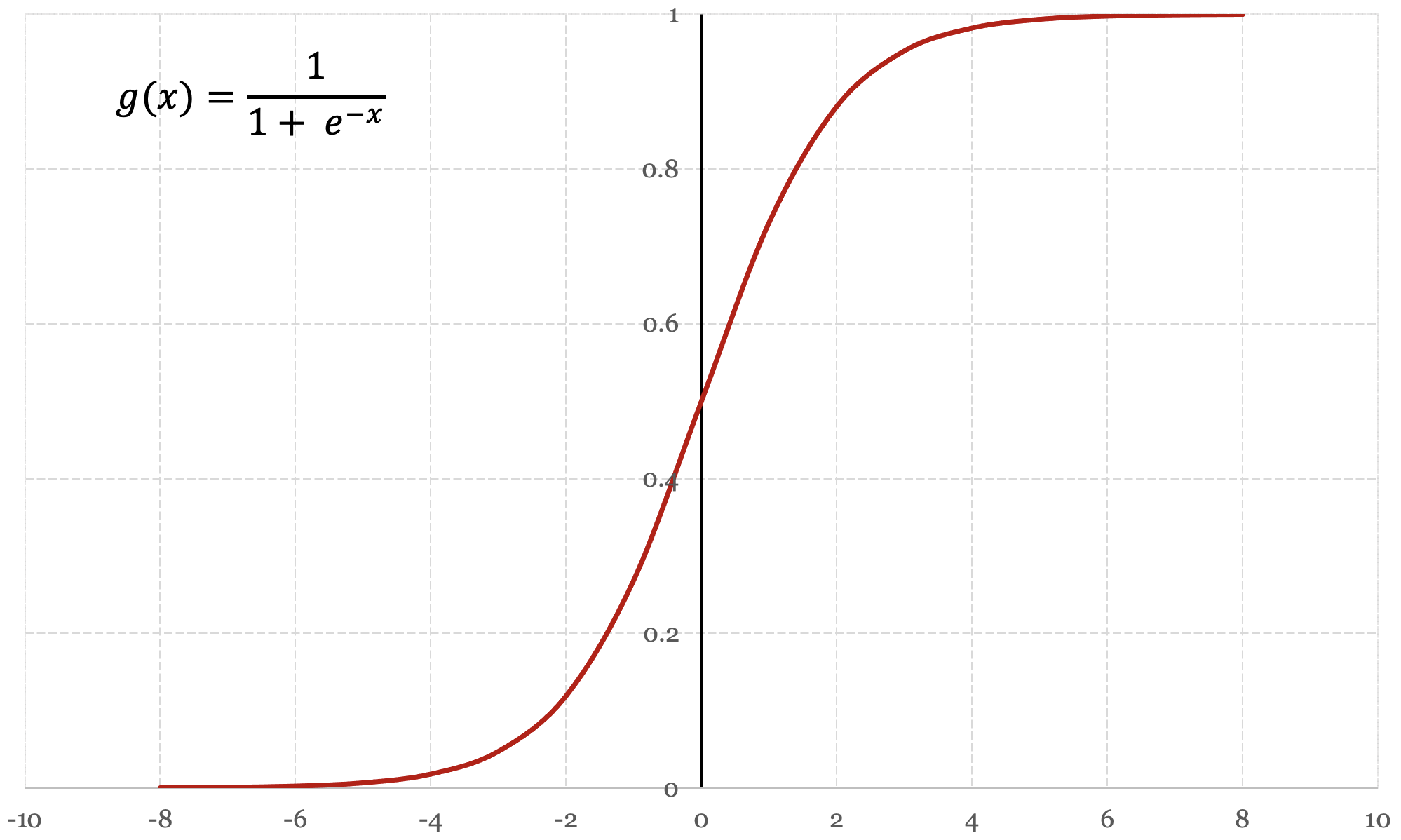
The logistic function, also referred to as the sigmoid function, is a function that neatly satisfies our requirements for classification. A logistic function is a type of bounded function that is defined for all input values x and has exactly one inflection point. The logistic function is defined as:

$$ g(x) = \frac{\mathrm{1} }{\mathrm{1} + e^x } $$

As an input value x approaches infinity, the output value of the logistic function approaches, or asymptotes towards the value 1. As an input value x approaches negative infinity, the output value of the logistic function approaches, or asymptotes towards the value 0. Figure 5-1 below presents a graph of the logistic function:

Figure 5-1: The logistic, or sigmoid function

The Hypothesis Function

The logistic function g(x) exhibits the characteristics we need for classification, so we’ll define our hypothesis function for classification as follows:

$$ h_\theta(x) = g(x) = \frac{\mathrm{1} }{\mathrm{1} + e^{-x} } $$

Since this function only outputs values ranging between 0 and 1 for any input value of x, it meets our requirements for a hypothesis function. In its current form, the hypothesis function can act as a predictor but it can’t yet model the relationship between input features and an output variable. To introduce this capability, we replace the input variable x in the logistic function with our previous definition of the hypothesis function for regression θ^Tx:

$$ h_\theta(x) = g(\theta^Tx) = \frac{\mathrm{1} }{\mathrm{1} + e^- \theta^Tx } $$

The logistic function g(x) is responsible for producing outputs between the range of 0 and 1, while linear or polynomial functions θ^Tx are responsible for modelling the relationship between input features and an output variable. We now have a model that can be trained and make predictions.

Hypothesis Function Interpretation

We’ve designed our hypothesis function h(x) so that it outputs a value between 0 and 1 for any input value of x. In binary classification, the output of the hypothesis function represents the probability that x belongs to exactly one of two categories. Since the probability could refer to either category, we need to choose one of them by default. Conventionally, we say that the output of the hypothesis function h(x) represents the probability that x belongs to the positive class (i.e. y = 1). We can express this convention more formally as:

$$ h_\theta(x) = P(y=1|x) $$

Put simply, the hypothesis function computes the probability that y = 1, given the input value x. To be even more specific, the output of the hypothesis function is influenced by the input value of a feature and the feature's learned parameter value θ.

$$ h_\theta(x) = P(y=1|x;\theta) $$

More formally, we say that the hypothesis function computes the probability that y = 1, given the input value x parameterized by θ.

As a concrete example, let’s assume we want to predict whether we should buy or sell a stock. We’ll say that sell is our negative class, and buy is our positive class. When the hypothesis function outputs a value of 0.72:

$ h(x) = 0.72 $

We should interpret this result as a 72% probability that we should buy the stock (i.e. y=1). Since binary classification consists of only two categories, we can also compute the probability that we should sell the stock (i.e. y=0). Since the sum of both probabilities must equal to 1, we can compute the probability that we should sell the stock as follows:

If there’s a 72% probability that we should buy the stock, there is a 28% probability that we should sell the stock.

The Decision Boundary

Now that we understand how to interpret the results from the hypothesis function, let’s get a better sense of what the hypothesis function is actually computing. The hypothesis function outputs a value between 0 and 1, which represents the probability that y = 1.

$$ h_\theta(x) = P(y=1|x;\theta) $$

What if the hypothesis function returns a value of exactly 0.5? This result tells us that there’s a 50% chance that y = 1, and consequently a 50% chance that y = 0. The positive class is conventionally chosen when this situation arises, and although the decision is somewhat arbitrary it’s good practice to remain consistent. We’ll formalize this convention by declaring:

$$ \text{when } h_\theta(x) \geq 0.5 \text{ then } y = 1 $$ $$ \text{when } h_\theta(x) < 0.5 \text{ then } y = 1 $$

Let’s revisit our logistic function to get some context around when these conditions occur.

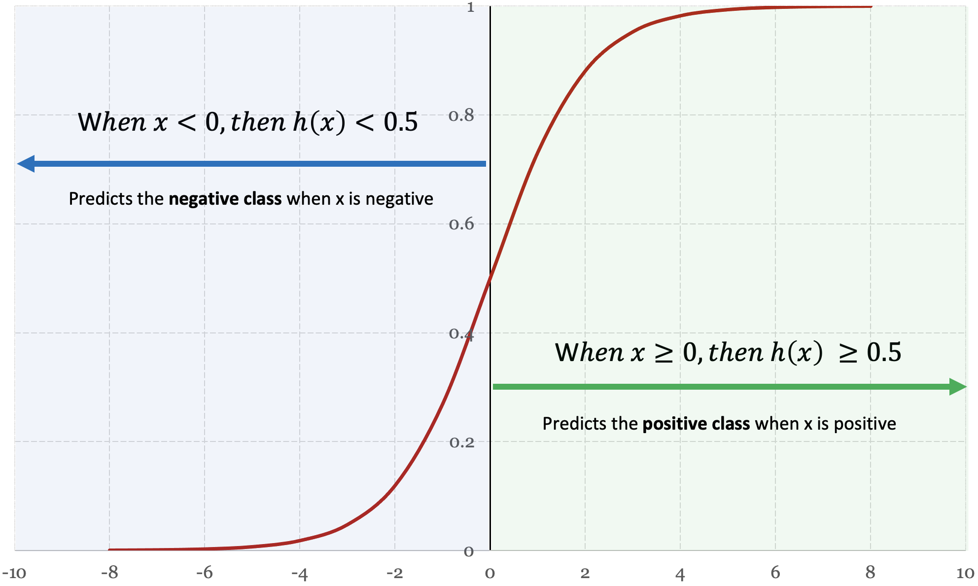
Figure 5-2: Hypothesis function h(x) output as a function of input variable x

Figure 5-2 shows when x is greater than or equal to zero, the hypothesis function h(x) outputs a value that is greater than or equal to 0.5. When x is less than zero, the hypothesis function h(x) outputs a value less than 0.5. Put simply, when x is a positive number then h(x) predicts the positive class, and when x is a negative number then h(x) predicts the negative class. Based on these observations, we can derive the following conclusion:

$$ \text{given } h_\theta(x) \geq 0.5 \text{ when } x \geq 0 $$ $$ \text{and } h_\theta(x) = g(\theta^Tx) $$ $$ \text{then } g(\theta^Tx) \geq 0.5 \text{ when } \theta^Tx \geq 0 $$

We’ve shown that whenever θ^Tx ≥ 0, the hypothesis function predicts the positive class, otherwise the hypothesis function predicts the negative class. This is what we refer to as the decision boundary – a well-defined boundary that objectively decides whether an input belongs to the positive class or negative class.

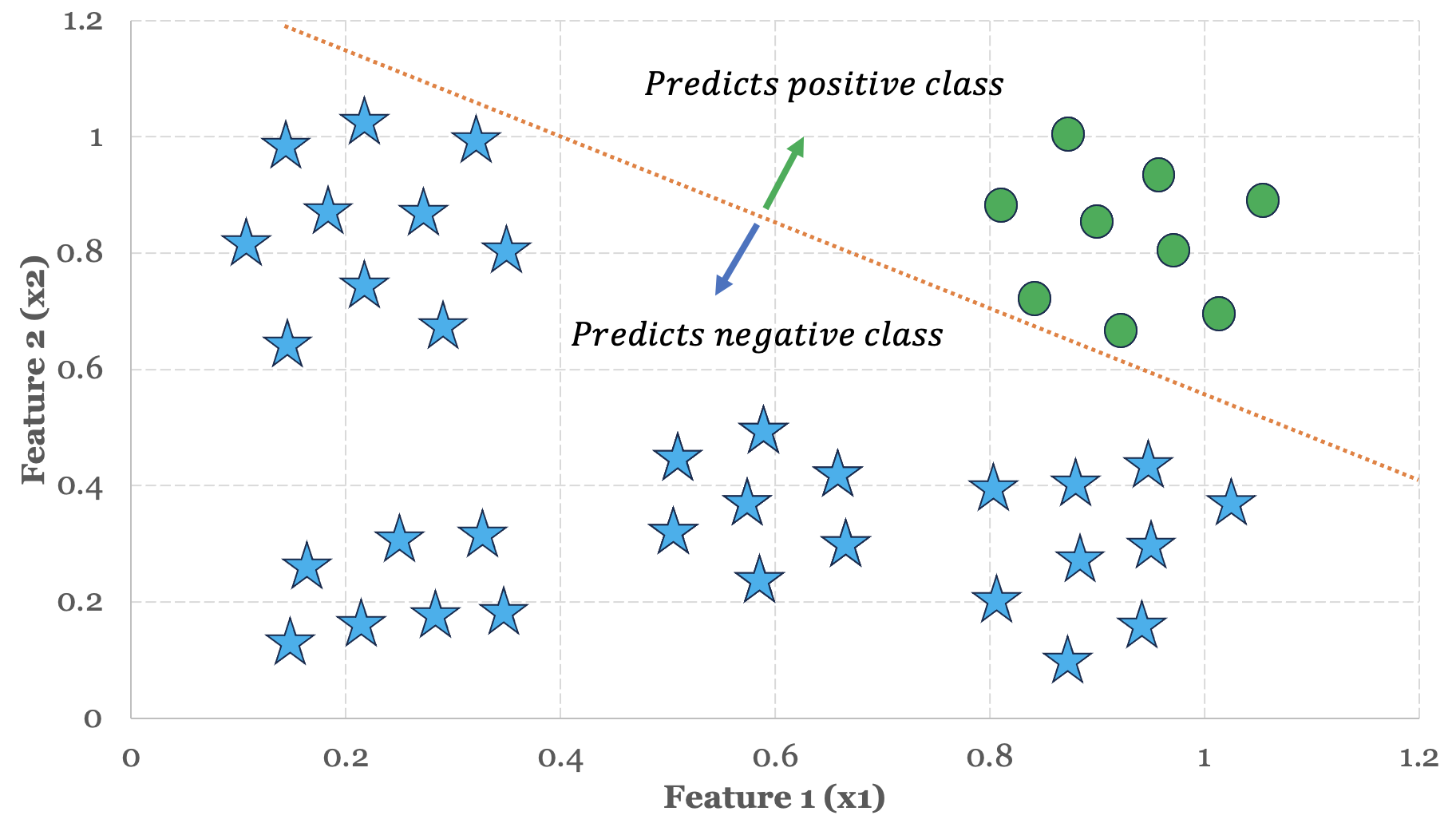
Let’s use this insight to understand how logistic regression makes predictions on a sample training set. In Figure 5-3 below, we have two distinct groups or clusters of data organized around two features.

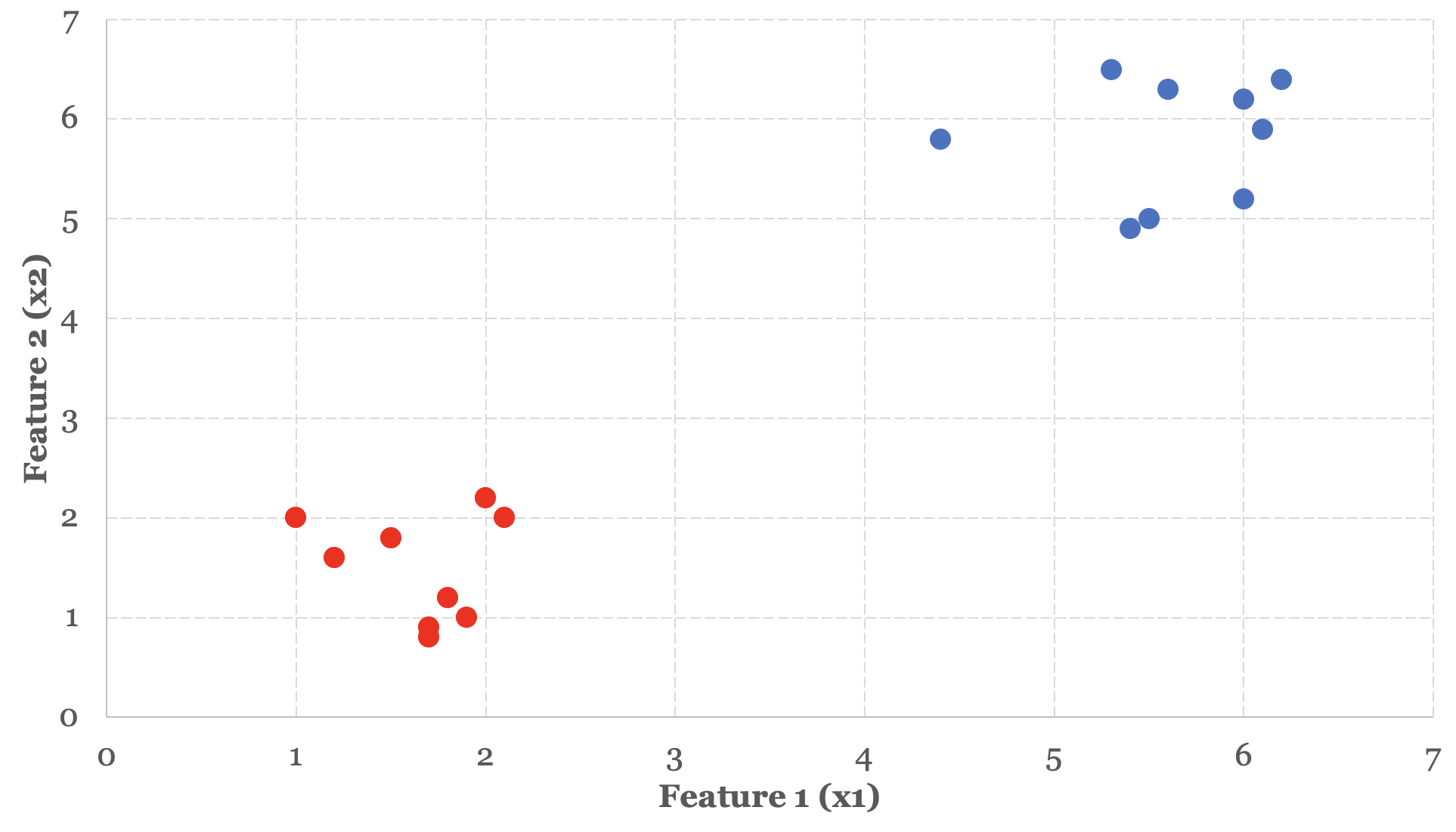
Figure 5-3: A sample data set for logistic regression

In the previous three chapters, we used linear and polynomial functions as a way to fit data. With classification models, we use linear and polynomial functions as a way to split data. In other words, we need to choose a function that can reasonably act as a dividing line to split, segregate or otherwise isolate these groups from one another. Based on the data presented in Figure 5-3, a linear function seems like an appropriate choice to act as our dividing line.

Since we have two features to model, we define a linear function as follows:

$ h_\theta(x) = \theta^Tx = \theta_0x_0 + \theta_1x_1 + \theta_2x_2 $

We define our decision boundary as:

$ \theta^Tx \geq 0 = \theta_0x_0 + \theta_1x_1 + \theta_2x_2 \geq 0 $

We know that whenever the following condition holds true for the input parameters x₀ to x₂, the logistic regression hypothesis function h(x) will predict the positive class:

$ \theta_0x_0 + \theta_1x_1 + \theta_2x_2 \geq 0 $

We haven’t discussed how our learning algorithm will fit the model parameters just yet, but let’s assume that the learning algorithm has produced the following parameter vector:

$ \theta = \begin{bmatrix}-6\\1\\1\end{bmatrix} $

If we use these parameter values in the boundary condition function, we end up with:

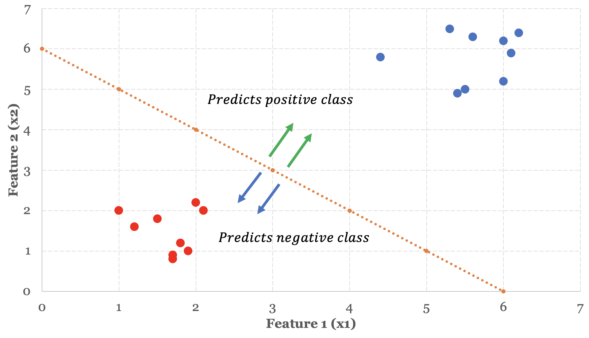
$ -6 + x_1 + x_2 \geq 0 $

We can rewrite this expression and see that with the parameter values -6, 1 and 1, the hypothesis function will predict a positive class whenever the sum of values x₁ and x₂ are greater than or equal to 6.

$ x_1 + x_2 \geq 6 $

Let’s plot the graph of x₁ + x₂ = 6 and see what our decision boundary looks like.

Figure 5-4: Sample data set for logistic regression with the decision boundary

The Cost Function

To date, we’ve been using the following cost function in our regression models:

$$ J(\theta) = \dfrac {1}{2m} \displaystyle \sum _{i=0}^m \left (\theta^Tx^{(i)} - y^{(i)} \right)^2 $$

The cost function produces a convex shape with a single global minima when we use it to evaluate the performance of linear or polynomial hypothesis functions. As we’ve previously discussed, gradient descent should only be used to minimize cost functions that produce a single global minima.

When we use this cost function to evaluate the performance of logistic functions, it ends up producing a non-convex shape with multiple local minima. Consequently, we need to develop a new cost function for logistic regression that is amenable to minimization by gradient descent.

Before we introduce the cost function for logistic regression, we want to present a simple training set that we might use to train a logistic regression model. This should provide some context around why the cost function for logistic regression looks a bit different from the cost function we’ve been using so far.

The table below contains a number of common industry standard performance indicators (PE Ratio, Operating Margin and Quick Ratio) along with a column that indicates whether we want to buy or sell stock in the company:

Table 5-1: Training set with company performance metrics

Company	PE Ratio	Operating Margin	Quick Ratio	Buy/Sell
AAPL	30	30.20%	0.81	1
AMZN	50.6	2.60%	0.7	0
GOOG	25.4	25.50%	2.14	0
MSFT	33.7	42.10%	1.75	1
TSLA	73.8	17.10%	1.07	0

The notable element in this table is the “Buy/Sell” column. In the previous chapters on regression models our goal was to predict the price of a stock, which happened to be an intrinsic part of the data sets we were studying. Consequently, we didn’t need to explicitly provide the regression models with labelled data. In our binary classification model, the decision to buy or sell stock in a company is data that we explicitly provide in the training set in order for the training algorithm to learn the relationship between our features and the decision to buy or sell.

Motivations for a new cost function

When predictions in our regression models strongly deviate from expected values, the cost function would compute an appropriately high cost. For example, if the predicted stock price for a training instance was \$10 and the actual stock price was \$50, the cost of this variation would be 40².

In logistic regression, the hypothesis function only outputs values ranging from 0 to 1. In a worst-case scenario, logistic regression could predict a value of 1 when the actual value is 0, or predict a value of 0 when the actual value is 1. In both cases, the cost of this deviation is exactly 1², for a total cost of exactly 1 in the worst-case scenario. This isn’t a particularly punitive cost, and consequently learning algorithms would struggle to learn or discover relationships with such moderate feedback. A cost function for logistic regression should amplify the cost of mistakes to make it easier for the learning algorithms to discover patterns and relationships.

With that context, let’s introduce the cost function for logistic regression and describe how it works in practice. The cost function for logistic regression is defined as:

$$ J(\theta) = \dfrac {1}{m} \displaystyle \sum _{i=0}^m \left (-y^{(i)}log(h_\theta(x^{(i)})) - (1 - y^{(i)})log(1 - h_\theta(x^{(i)}) \right) $$

There’s a bit to unpack here, but this cost function is not necessarily as complicated as it first appears. The first thing we want to show is the cost function is actually composed of two simpler cost functions.

If you refer back to Table 5-1, our first training instance APPL has an expected “Buy/Sell” value of 1, or in other words y = 1. Let’s plug in the value y = 1 and see what the cost function looks like:

$$ J(\theta) = \dfrac {1}{m} \displaystyle \sum _{i=0}^m \left (-(1)log(h_\theta(x^{(i)})) - (1 - 1)log(1 - h_\theta(x^{(i)}) \right) $$

You can see that when y = 1, the second term in this equation cancels out entirely since 1 - 1 = 0, so we end up with the following cost function in cases where y = 1:

$$ J(\theta) = \dfrac {1}{m} \displaystyle \sum _{i=0}^m -log(h_\theta(x^{(i)})) $$

Our second training instance AMZN has an expected “Buy/Sell” value of 0, or in other words y = 0. Let’s plug in the value y = 0 and see what the cost function looks like:

$$ J(\theta) = \dfrac {1}{m} \displaystyle \sum _{i=0}^m \left (-(0)log(h_\theta(x^{(i)})) - (1 - 0)log(1 - h_\theta(x^{(i)}) \right) $$

You can see that when y = 0, the first term in this equation cancels out entirely, so we end up with the following cost function in cases where y = 0:

$$ J(\theta) = \dfrac {1}{m} \displaystyle \sum _{i=0}^m -log(1 - h_\theta(x^{(i)})) $$

This shows that the cost function for logistic regression is actually composed of two distinct cost functions: one cost function for when y = 1, and another cost function for when y = 0. The cost function automatically “collapses” into the appropriate function based on the value of y, so this isn’t a behaviour that you need to manage or implement yourself.

The second thing we want to show is how logarithmic functions can be used to amplify the cost of a wrong prediction. First, let’s take the case where y = 1 and the cost of an individual training instance x⁽ⁱ⁾ is:

$$ -log(h_\theta(x^{(i)})) $$

Remembering that the hypothesis function for logistic regression is the logistic or sigmoid function, let’s plot the log of our hypothesis function.

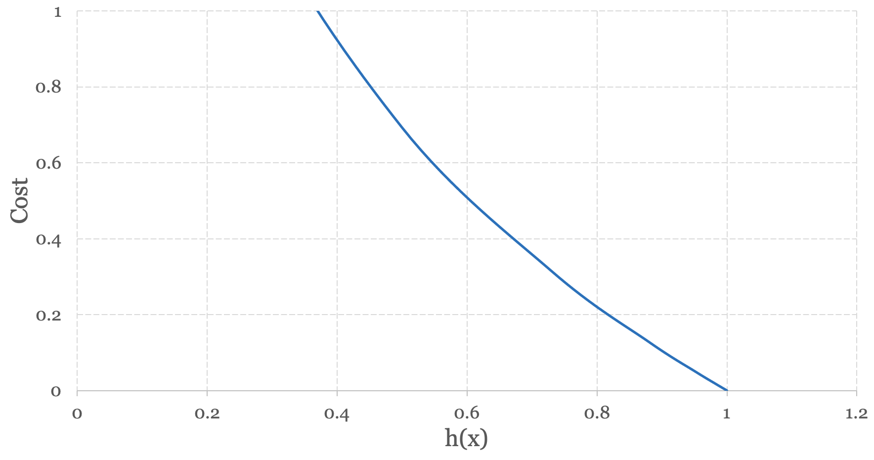
Figure 5-5: Cost -log(h(x)) as a function of h(x)

When h(x) outputs a value approaching 1, the cost approaches 0. When h(x) outputs a value approaching 0, the cost grows exponentially. In other words, when the hypothesis function makes the correct prediction (i.e. y = 1) the cost associated with the prediction approaches zero. When the hypothesis function makes the wrong prediction (i.e. y = 0) the cost approaches infinity.

Now let’s take the case where y = 0 and the cost of an individual training instance x(i) is:

$$ -log(h_\theta(1 - x^{(i)})) $$

When we plot the log of this function we end up with Figure 5-6 below:

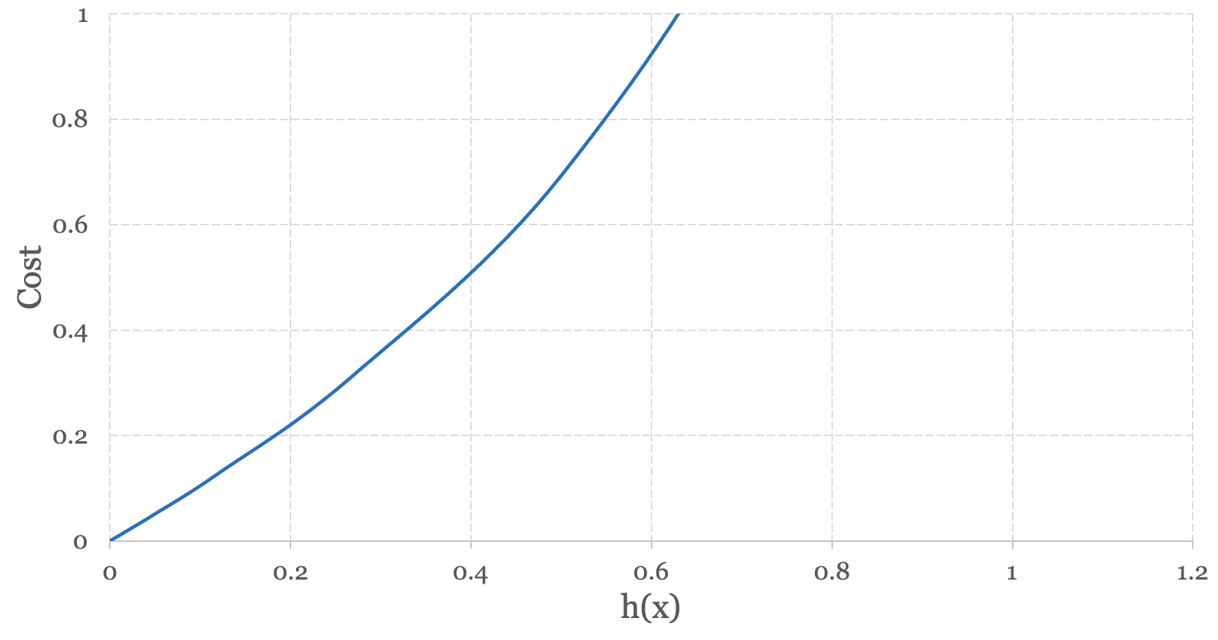
Figure 5-6: Cost -log(1 - h(x)) as a function of h(x)

In this case, when h(x) outputs a value approaching 0, the cost approaches 0. When h(x) outputs a value approaching 1, the cost grows exponentially. In other words, when the hypothesis function makes the correct prediction (i.e. y = 0) the cost associated with the prediction approaches zero. When the hypothesis function makes the wrong prediction (i.e. y = 1) the cost approaches infinity.

By taking the log of our respective cost function we can amplify the cost, or better penalize mistakes when our learning algorithm makes the wrong predictions during training.

One minor semantical note with respect to the logistic regression cost function. Conventionally the negative signs within the cost function are extracted outside of the cost function, so more commonly you’ll see definitions of the cost function defined as:

$$ J(\theta) = -\dfrac {1}{m} \displaystyle \sum _{i=0}^m \left (y^{(i)}log(h_\theta(x^{(i)})) + (1 - y^{(i)})log(1 - h_\theta(x^{(i)}) \right) $$

While stylistically different, it is functionally equivalent to the original definition provided at the beginning of the chapter.

Gradient Descent

To date, we’ve been using the following gradient descent algorithm in our regression models:

Repeat simultaneously until convergence, for j = 0 to j = n: {

$$ \theta_j := \theta_j - \alpha \dfrac {1}{m} \displaystyle \sum _{i=0}^m \left (\theta_0x_0^{(i)} + ... + \theta_nx_n^{(i)} - y^{(i)} \right)x_j^{(i)} $$

}

As much as the cost function has changed in logistic regression, the gradient descent algorithm has not. In fact, we can use gradient descent in logistic regression in the exact same way that we’ve used it in our regression models. You simply need to substitute the reference to the hypothesis function h(x) with the hypothesis function that we’ve developed for logistic regression.

$$ h_\theta(x) = \frac{\mathrm{1} }{\mathrm{1} + e^- \theta^Tx } $$

Now that we’ve defined the hypothesis function, cost function and gradient descent for logistic regression you have all of the tools you need to implement a binary classification model. In the next section, we’ll extend the ideas of binary classification to show you how you can implement multiclass classification models.

Multiclass Classification

Multiclass classification is a model that can classify input data into an arbitrarily large number of classes or categories. Given an input x, multiclass classification outputs the probability that x belongs to a specific category, in the same way that binary classification does. We represent these categories formally as:

$ y ∈ \{C_1, C_2 ... C_k\} $

Multiclass classification leverages all of the machinery of binary classification and uses a technique called One vs. All to produce one binary classifier for each category or class in your model.

There are a number of practical applications of multiclass classification. When we introduced binary classification, we were limited in our ability to characterize our interest in equity investments - we had two categories to choose from, buy or sell. In multiclass classification, we can apply a more meaningful characterization model that is commonly used by market analysts – sell, underperform, hold, outperform and buy.

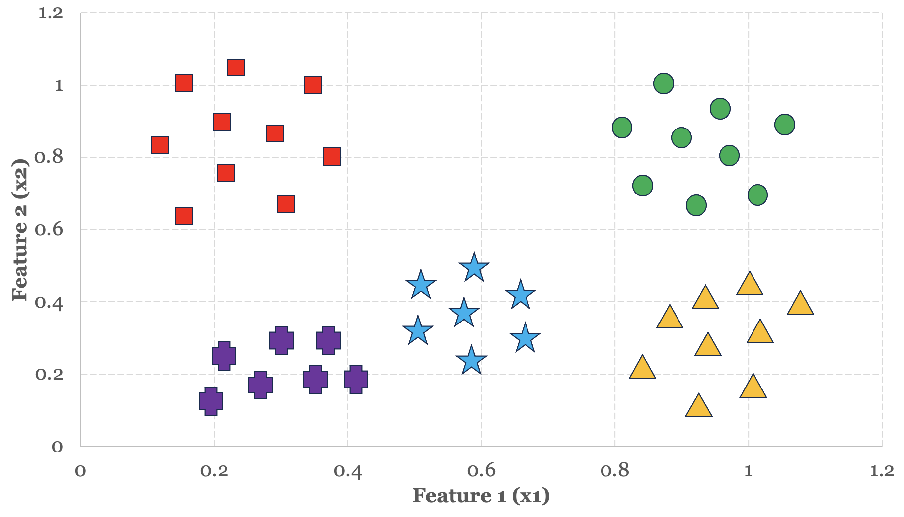
As a practical example, let’s apply the One vs. All technique using these five categories to see how this technique works. In Figure 5-7 below, we have five distinct groups or clusters of data organized around two features. For the sake of this exercise, let’s say:

The red group represents the sell training instances.
The green group represents the buy training instances.
The blue group represents the underperform training instances.
The yellow group represents the outperform training instances.
The purple group represents the hold training instances.

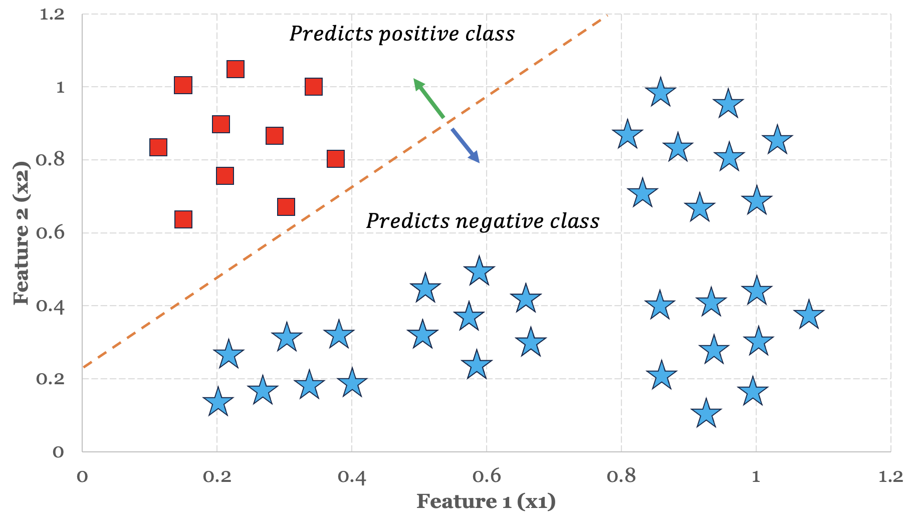
Figure 5-7: The five distinct equity characterization groups

We start by targeting or isolating one particular group. Let’s begin by isolating the red sell group first. In our training set, we assign y = 1 to all sell training instances, and we assign y = 0 to all other training instances. As a result, we end up with two distinct groups – the sell group and the not sell group. We then train our model using binary classification and retain the model - which we refer to as a classifier. The figure below shows how the red group is isolated from the remaining groups via the decision boundary.

Figure 5-8: One vs. All targeting the red (sell) group

We repeat this process for every group in our model. As one more example, let’s isolate the green buy group next. In our training set, we assign y = 1 to all buy training instances, and we assign y = 0 to all other training instances. As a result, we end up with two distinct groups – the buy group and the not buy group. We then train a brand new model using binary classification and retain this model as well. Figure 5-9 below shows how the green buy group is isolated from the remaining groups via the decision boundary.

Figure 5-9: One vs. All targeting the green (buy) group

Once complete you will have five distinct models or classifiers, each one tuned to identify one particular group. To make a prediction, create an “entry point” function that acts as a facade over each of the classifiers. When invoked, the function iterates over each classifier and returns the result from the classifier whose probability is greatest. With a little bit of data wrangling, you now know how to implement a multiclass classification model.

Build the Logistic Regression Model

We’ve published an implementation of the logistic regression model on GitHub.

If you would like to implement, train and run this logistic regression model yourself, feel free to use the source code as a reference and run the software to see how training and running the model works in practice. Documentation related to building, training and running the model can be found on GitHub as well.

https://github.com/build-thinking-machines/logistic-regression